Lecture 16. Linear model with a classifying factor 2020 (1) A - PowerPoint PPT Presentation
Lecture 16. Linear model with a classifying factor 2020 (1) A simple anova (2) Two breeds of sheep Black Welsh A measurement is taken on a 6.6 10.4 random sample of ve animals 8.1 9.8 from each of two breeds. Is 7.6 11.0 there
Lecture 16. Linear model with a classifying factor 2020
(1) A simple anova
(2) Two breeds of sheep Black Welsh A measurement is taken on a 6.6 10.4 random sample of ˛ve animals 8.1 9.8 from each of two breeds. Is 7.6 11.0 there evidence for a di¸erence 6.9 10.6 between breeds? 8.3 9.2
(3) An indicator variable Breed X Y Black 0 6.6 Black 0 8.1 Black 0 7.6 Black 0 6.9 Black 0 8.3 Welsh 1 10.4 Welsh 1 9.8 Welsh 1 11.0 Welsh 1 10.6 Welsh 1 9.2 X is an indicator variable for the Welsh breed.
(4) An indicator variable Set X = 0 for each measurement on a Blackface animal and X = 1 for each measurement on a Welsh animal. The linear model E ( Y ) = b 0 + b 1 X assigns means to breeds as follows: Breed X b 0 + b 1 X Black 0 b 0 Welsh 1 b 0 + b 1 b 0 : mean value for Blackface breed b 1 : di¸erence between Welsh and Blackface Null hypothesis b 1 = 0 is equivalent to ’no di¸erences between breeds’.
(5) Using lm (with indicator variable) Y <- 0.1 * c(66,81,76,69,83,104,98,110,106,92) X <- rep(0:1, each = 5) fit <- lm(Y ˜ X) summary(fit) anova(fit) t statistic (from summary) or F statistic (from anova) tests b 1 = 0 (no di¸erence between breeds).
(6) Using lm (with factor) Y <- 0.1 * c(66,81,76,69,83,104,98,110,106,92) Breed <- gl(2,5, labels = c(’Black’,’Welsh’)) fit <- lm(Y ˜ Breed) summary(fit) t statistic (from summary) or F statistic (from anova) tests b 1 = 0 (no di¸erence between breeds). Output is identical to that obtained using an indicator variable (apart from labelling of estimates).
(7) Output from summary and anova Output from summary: Estimate SE t Intercept 7.5 0.3233 23.201 BreedWelsh 2.7 0.4572 5.906 Output from anova: DF SSQ MSQ F Breed 1 18.225 18.2250 34.88 Residuals 8 4.180 0.5225
(8) Three breeds of sheep Three breeds of sheep: Blackface, Welsh, and the Blackface ˆ Welsh cross. A measurement is taken on a random sample of ˛ve animals from each breed. Is there evidence for a di¸erence between breeds? Black Welsh Cross 6.6 10.4 7.0 8.1 9.8 9.3 7.6 11.0 8.4 6.9 10.6 7.6 8.3 9.2 9.7
(9) Two indicator variables X and Z are indicators for the Welsh and Cross breeds. The linear model E ( Y ) = b 0 + b 1 X + b 2 Z assigns means to breeds as follows: Breed X Z b 0 + b 1 X + b 2 Z Black 0 0 b 0 Welsh 1 0 b 0 + b 1 Cross 0 1 b 0 + b 2 b 0 : mean value for Blackface breed b 1 : di¸erence between Welsh and Blackface b 2 : di¸erence between Cross and Blackface Null hypothesis b 1 = b 2 = 0 is equivalent to ’no di¸erences among breeds’.
(10) Parameter estimates Parameter estimates: ^ b 0 = — ^ b W = — Y W ` — ^ b C = — Y C ` — Y B ; Y B ; Y B Fitted value ^ b 0 + ^ b W X + ^ b C Z is Y B = ^ — b 0 (Blackface observation) Y W = ^ — b 0 + ^ b W (Welsh observation) Y C = ^ — b 0 + ^ b C (Cross observation) Fitted value for an observation is the mean observation for its breed.
(11) Sums of squares Anova equation (for multiple regression): Y ) 2 = Y ) 2 + X ( Y ` — X (^ Y ` — X ( Y ` ^ Y ) 2 Regression sum of squares ( S B ) is the mean-corrected sum of squares of the three ˛tted values, weighted by the size of sample. Residual sum of squares ( S W ) is the sum of the mean-corrected sums of squares within each breed.
(12) Anova table With k groups, and a total of N = nk observations, regression and residual sums of squares have k ` 1 and N ` k d.f. Anova table is calculated in the usual way: Source DF SSQ MSQ F Between k ` 1 S B M B M B =M W Within N ` k S W M W M W (previously S 2 ) estimates the residual variance.
(13) The ’sheep’ data frame Breed Cu X Z Black 6.6 0 0 Black 8.1 0 0 Black 7.6 0 0 Black 6.9 0 0 Black 8.3 0 0 Welsh 10.4 1 0 Welsh 9.8 1 0 Welsh 11.0 1 0 Welsh 10.6 1 0 Welsh 9.2 1 0 Cross 7.0 0 1 Cross 9.3 0 1 Cross 8.4 0 1 Cross 7.6 0 1 Cross 9.7 0 1
(14) Using lm (with factor) library(sda) # if necessary fit <- lm(Cu ˜ Breed, data = sheep) anova(fit) Alternatively: fit <- aov(Cu ˜ Breed) summary(fit)
(15) ANOVA Anova table for the sheep data is Source DF SSQ MSQ F Between breeds 2 18.90 9.450 12.22 Within breeds 12 9.28 0.773 Total 14 28.18 F = 12 : 22 on 2 and 12 d.f. ( P < 0 : 01). Di¸erences between breeds are established beyond reasonable doubt.
END OF LECTURE
Lecture 17. Comparisons among means 2020
(16) ANOVA Anova table for the sheep data is Source DF SSQ MSQ F Between breeds 2 18.90 9.450 12.22 Within breeds 12 9.28 0.773 Total 14 28.18 F = 12 : 22 on 2 and 12 d.f. ( P < 0 : 01). Di¸erences between breeds are established beyond reasonable doubt.
(17) Comparing two means Mean values for each breed: Black Welsh Cross 7.5 10.2 8.4 Estimated standard error of a di¸erence between two means based on n 1 and n 2 observations is q M W (1 =n 1 + 1 =n 2 ) where M W is the within-group mean square. For the sheep data, M W = 0 : 773, n 1 = n 2 = 5, and standard error of di¸erence between any two breed means is 0.556.
(18) Output from summary Estimate Std.Error t.value (Intercept) 7.5000 0.3933 19.071 BreedCross 0.9000 0.5562 1.618 BreedWelsh 2.7000 0.5562 4.855
(19) Comparing two means Comparison Estimate SE t Welsh ` Blackface 2.7 0.556 4.86 Cross ` Blackface 0.9 0.556 1.62 Welsh ` Cross 1.8 0.556 3.24 (Upper 2.5% point of t on 12 d.f. is 2.179). A 95% con˛dence interval for Welsh ` Blackface is 2.7 ˚ 2.179 ˆ 0.556, or (1.49, 3.91).
(20) More general comparisons The ’contrast’ C = a 1 — Y 1 + a 2 — Y 2 + ´ ´ ´ + a k — Y k has estimated standard error v @ a 2 + a 2 + ´ ´ ´ + a 2 u 0 1 u 1 2 k t M W u A n 1 n 2 n k Under H 0 : E ( C ) = 0, the statistic obtained by dividing C by its estimated standard error has an t distn with N ` k degrees of freedom. Usually a 1 + a 2 + ´ ´ ´ + a k = 0.
(21) Example of a contrast A possible contrast of interest is 0 : 5 ˜ (— Y B + — Y W ) ` — Y C . Value of this contrast is 0 : 5 ˆ (7 : 5 + 10 : 2) ` 8 : 4 = 0 : 45, with estimated standard error q 0 : 773(1 = 20 + 1 = 20 + 1 = 5) = 0 : 48155. T statistic is 0 : 45 = 0 : 48155 = 0 : 93 with 12 d.f. Test result is not signi˛cant. A 95% interval estimate for the contrast is 0 : 45 ˚ 2 : 179 ˆ 0 : 48155, or ( ` 0 : 60 ; +1 : 50).
(22) Fruit ‚ies Bristle counts on 20 fruit ‚ies, ˛ve ‚ies in each of four genotype classes. A B C D 16 8 9 5 12 12 12 8 16 7 11 8 11 9 10 7 15 12 8 9 genotype class means A B C D (14.0) (9.6) (10.0) (7.4)
(23) Fruit ‚ies ANOVA of the fruit ‚y data shows highly signi˛cant di¸erences among genotype classes (P < 0.001). We could continue the analysis by producing a table of six pairwise comparisons, A versus B, etc, but this would not shed much light on the data. Additional information on the genotype classes allows a more informative analysis.
(24) Cy and Me mutations The key to a more informative analysis is knowing that genotype classes A { D are determined by presence (+) or absence ( ` ) of two mutations, Cy and Me. A B C D Cy ` ` + + Me ` + ` +
(25) Informative contrasts A B C D Cy ` ` + + Me ` + ` + Cy ˆ Me + ` ` + (C ` A) estimates the Cy e¸ect when Me is absent, (D ` B) estimates the Cy e¸ect when Me is present. The Cy contrast estimates the sum (or average) of these two conditional e¸ects. (C ` A+B ` D) estimates the di¸erence between the two conditional e¸ects (the interaction Cy ˆ Me).
(26) An interaction plot 14 mutation Me absent present number of bristles 12 10 8 absent present mutation Cy
(27) Anova with two factors Instead of setting up one factor (genotype) with four levels, set up two factors (Cy and Me), each with two levels (’present’, ’absent’). Anova based on bristles ‰ Cy + Me + Cy:Me has three single d.f. sums of squares, for the average Cy e¸ect, the average Me e¸ect, and the interaction. F ratios are the squares of t statistics obtained from contrasts, and the three sums of squares add up to the ’genotypes’ sum of squares with 3 d.f. Model formula can also be written bristles ‰ Cy * Me
END OF LECTURE
Lecture 18. The random e¸ects model 2020
(28) Random e¸ects model As previously we have k groups of size n , total number of observations N = nk . Random e¸ects model: Y i = m + U r + e i where r is the group which contains observation i . U 1 : : : U k and e 1 : : : e N are independent r.v.s normally distributed with zero mean and var( U ) = ff 2 var( e ) = ff 2 B ; W : Total variance of a single observation ff 2 B + ff 2 W is partitioned into components ff 2 B and ff 2 W .
(29) Expected mean squares Source DF MSQ E(MSQ) ff 2 W + nff 2 Between groups k ` 1 M B B ff 2 Within groups N ` k M W W F = M B =M W tests H 0 : ff 2 B = 0. Y estimates m , with variance ( ff 2 — W + nff 2 B ) =N . q Estimated standard error is E = M B =N . Interval estimate for m is — Y ˚ kE where k is an upper quantile of t with k ` 1 d.f.
Recommend
More recommend
Explore More Topics
Stay informed with curated content and fresh updates.
