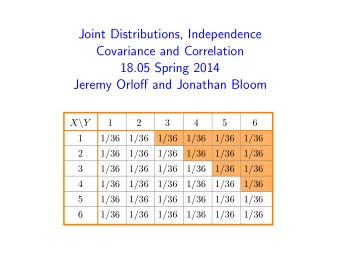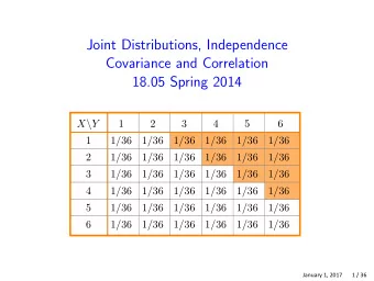
Lecture 16 : Independence, Covariance and Correlation of Discrete - PDF document

Lecture 16 : Independence, Covariance and Correlation of Discrete Random Variables 0/ 31

Definition Two discrete random variables X and Y defined on the same sample space are said to be independent if for nay two numbers x and y the two events ( X = x ) and ( Y = y ) are independent ⇔ and (*) 1/ 31 Lecture 16 : Independence, Covariance and Correlation of Discrete Random Variables

Now (*) say the joint pmf P X , Y ( x , y ) is determined by the marginal pmf ’s P X ( x ) and P Y ( y ) by taking the product. Problem In case X and Y are independent how do you recover the matrix (table) representing P X , y ( x , y ) from its margins? 2/ 31 Lecture 16 : Independence, Covariance and Correlation of Discrete Random Variables

Let’s examine the table for the standard example ❍❍❍❍❍ Y 0 1 2 3 X ❍ 1 2 1 1 0 0 8 8 8 2 1 2 1 1 1 0 8 8 8 2 1 3 3 1 8 8 8 8 Note that X = ♯ of heads on the first toss Y = total ♯ of heads in all three tosses So we wouldn’t expect X and Y to be independent (if we know X = 1 that restricts the values of Y .) 3/ 31 Lecture 16 : Independence, Covariance and Correlation of Discrete Random Variables

Lets use the formula (*) It says the following. Each position inside the table corresponds to two positions on the margins 1 Go to the right 2 Go Down So in the picture 1 If we go right we get 1 2 2 If we go down we get 3 8 4/ 31 Lecture 16 : Independence, Covariance and Correlation of Discrete Random Variables

If X and Y are independent then the formula (*) says the entry inside the table is obtain by multiplying 1 and 2 So if X and Y wave independent then we would set ❍❍❍❍❍ Y 0 1 2 3 X ❍ 1 3 3 1 1 0 ( ♯ ) 16 16 16 16 2 1 3 3 1 1 1 16 16 16 16 2 1 3 3 1 8 8 8 8 5/ 31 Lecture 16 : Independence, Covariance and Correlation of Discrete Random Variables

So as we expected for the basic example X and Y are not independent. From (*) on page 5 we have ❍❍❍❍❍ Y 0 1 2 3 X ❍ (*) 1 2 1 0 0 8 8 8 1 2 1 1 0 8 8 8 This is not the same as ( ♯ ). 6/ 31 Lecture 16 : Independence, Covariance and Correlation of Discrete Random Variables

Covariance and Correlation In the “real world” e.g., the newspaper one often hears (reeds) that two quantities are correlated . This word is often taken to be synonymous with causality . This is not correct and the difference is extremely important even in reel life. Here are two real word examples of correlations. 1 Being rich and driving on expensive car. 2 Smoking and lung cancer. In the first case there is no causality whereas it is critical that in the second there is. 7/ 31 Lecture 16 : Independence, Covariance and Correlation of Discrete Random Variables

Statisticians can observe correlations (say for 2) but not causalities. Now for the mathematical theorem Covariance Definition Suppose X and Y are discrete and defined on the same sample space. Then the covariance Cov ( X , Y ) between X and Y is defined by Cov ( X , Y ) = E (( X − µ X )( Y − µ Y )) � = ( x − µ X )( y − µ Y ) P X , Y ( x , y ) x , y 8/ 31 Lecture 16 : Independence, Covariance and Correlation of Discrete Random Variables

Remark � ( X − µ X ) 2 � Cov ( X , X ) = E = V ( X ) There is a shortcut formula for covariance. Theorem (Shortcut formula) Cov ( X , Y ) = E ( XY ) − µ X µ Y Remark If you put X = Y you get the shortcut formula for the variance V ( X ) = E ( X 2 ) − µ 2 X 9/ 31 Lecture 16 : Independence, Covariance and Correlation of Discrete Random Variables

Recall that X and Y are independent ⇔ P X , Y ( x , y ) = P X ( x ) P Y ( y ) . Theorem X and Y are independent Cov ( X , Y ) = 0 ⇒ (the reverse implication does not always hold). Proof � E ( XY ) = xyP X , Y ( x , y ) x , y 10/ 31 Lecture 16 : Independence, Covariance and Correlation of Discrete Random Variables

Proof (Cont.) Now if X and Y are independent then P X , Y ( x , y ) = P X ( x ) P Y ( y ) So � E ( XY ) = xyP X ( x ) P Y ( y ) x , y � � = × P X ( x ) yP y ( y ) x y = µ X µ Y Hence Cov ( X , Y ) = µ X µ Y − µ X µ Y = 0 � 11/ 31 Lecture 16 : Independence, Covariance and Correlation of Discrete Random Variables

Corelation � � Let X and Y be as before and suppose σ X = V ( X ) and σ Y = V ( Y ) be their respective standard deviations. Definition The correlation, Corr ( X , Y ) or ρ X , Y or just ρ , is defined by ρ X , Y = Cov ( X , Y ) σ X σ Y 12/ 31 Lecture 16 : Independence, Covariance and Correlation of Discrete Random Variables

Proposition − 1 ≤ ρ X , Y ≤ 1 Theorem The meaning of correlation. 1 e X , Y = 1 ⇔ Y = aX + b with a > 0 “perfectly correlated” 2 P X , Y = − 1 ⇔ Y = aX + b with a < 0 “perfectly anticorrelated” 3 X and Y are independent ⇒ ρ X , Y = 0 but not conversely as we will see Pg. 18-21. 13/ 31 Lecture 16 : Independence, Covariance and Correlation of Discrete Random Variables

A Good Citizen’s Problem Suppose X and Y are discrete with joint pmf given by that of the basic example (*) ❍❍❍❍❍ Y 0 1 2 3 X ❍ 1 2 1 0 0 8 8 8 1 2 1 1 0 8 8 8 (i) Compute Cov ( X , Y ) (ii) Compute ρ X , Y Solution We first need the marginal distributions. 14/ 31 Lecture 16 : Independence, Covariance and Correlation of Discrete Random Variables

Solution (Cont.) X 0 1 1 1 P ( X = x ) 2 2 � � 1 , 1 so E ( X ) = 1 2 , V ( X ) = 1 4 and σ X = 1 So X ∼ Bin 2 2 Y 0 1 2 3 1 3 3 1 P ( Y = y ) 8 8 8 8 √ � � 3 , 1 so E ( Y ) = 3 2 , V ( X ) = 3 3 So Y ∼ Bin 4 so σ Y = 2 . 2 Now we need E ( XY ) (the hard part) � E ( XY ) = xy P ( X = x , Y = y ) xy Trick - We are summing over entries in the matrix times xy so potentially eight terms. 15/ 31 Lecture 16 : Independence, Covariance and Correlation of Discrete Random Variables

Solution (Cont.) But the four terms from first row don’t contribute because x = 0 so xy = 0 . Also the first term in the second row doesn’t contribute since y = 0 . So there are only three terms. � 1 � � 2 � � 1 � E ( XY ) = ( 1 )( 1 ) + ( 1 )( 2 ) + ( 1 )( 3 ) 8 8 8 = 1 8 [ 1 + 4 + 3 ] = 8 8 = 1 So Cov ( X , Y ) = E ( XY ) − µ X µ Y � 1 � � 3 � = 1 = 1 − 2 2 4 16/ 31 Lecture 16 : Independence, Covariance and Correlation of Discrete Random Variables

Solution (Cont.) (ii) ρ X , Y = Cov ( X , Y ) σ X σ Y 1 / 1 / ✁ 4 4 � = = � � √ √ � 1 3 / ✁ 4 3 2 2 √ = − 1 3 = √ 3 3 17/ 31 Lecture 16 : Independence, Covariance and Correlation of Discrete Random Variables

A cool counter example We need an example to show Cov ( X , Y ) = 0 � X and Y are independent So we need to describe a pmf . Here is its “graph” ( ♯ ) What does this mean. The corner points (with the zeroes) are ( 1 , 1 ) , ( 1 , − 1 ) , ( − 1 , − 1 ) and ( − 1 , 1 ) (clockwise) 18/ 31 Lecture 16 : Independence, Covariance and Correlation of Discrete Random Variables

and of course the origin. Here is the bar graph The vertical spikes have height 1 / 4 . The matrix of the pmf is ❍❍❍❍❍ Y − 1 0 1 X ❍ 1 1 − 1 0 0 4 4 (*) 1 1 1 0 0 4 4 2 1 1 1 0 0 4 4 1 1 1 4 2 4 I have given the marginal distributions. 19/ 31 Lecture 16 : Independence, Covariance and Correlation of Discrete Random Variables

Here are the tables for the marginal distributions X − 1 0 1 E ( X ) = 0 1 1 1 P ( X = x ) 4 2 4 Y − 1 0 1 E ( Y ) = 0 1 1 1 P ( Y = y ) 4 2 4 Now for the covariance. Here is the really cool thing. Every term in the Formula for E ( XY ) so E ( XY ) is the sum of nine zeroes so E ( XY ) = 0. So Cov ( X , Y ) = E ( XY ) − E ( X ) E ( Y ) = 0 − ( 0 )( 0 ) 20/ 31 Lecture 16 : Independence, Covariance and Correlation of Discrete Random Variables

But X and Y are not independent because if we go from the outside in we get ❍❍❍❍❍ Y − 1 0 1 X ❍ 1 / 1 / 1 / 1 / − 1 16 8 16 4 (**) 1 / 1 / 1 / 1 / 0 8 4 8 2 1 / 1 / 1 / 1 / 1 16 8 16 4 1 / 1 / 1 / 4 2 4 (*) � (**). So X and Y are not independent. 21/ 31 Lecture 16 : Independence, Covariance and Correlation of Discrete Random Variables

It turns out the picture ( ♯ ) gives us another counter example. Consider the following three events So A = { ( 0 , 1 ) , ( − 1 , 1 ) , ( − 1 , 0 ) } B = { ( 0 , 1 ) , ( 0 , 0 ) , ( 0 , − 1 ) } C = { ( 0 , 1 ) , ( 1 , 1 ) , ( 1 , 0 ) } 22/ 31 Lecture 16 : Independence, Covariance and Correlation of Discrete Random Variables

We claim 1 A , B , C are pairwise independent but not independent. That is P ( A ∩ B ) = P ( A ) P ( B ) P ( A ∩ C ) = P ( A ) P ( C ) P ( B ∩ C ) = P ( B ) P ( C ) but P ( A ∩ B ∩ C ) = P ( A ) P ( B ) P ( C ) 23/ 31 Lecture 16 : Independence, Covariance and Correlation of Discrete Random Variables

Let’s check this P ( A ) = P ( { ( 0 , 1 ) , ( − 1 , 1 ) , ( − 1 , 0 ) } = 1 2 P ( B ) = P ( { ( 0 , 1 ) , ( 0 , 0 ) , ( 0 , − 1 ) } = 1 2 P ( C ) = P ( { ( 0 , 1 ) , ( 1 , 1 ) , ( 1 , 0 ) } = 1 2 A ∩ B = { ( 0 , 1 ) } A ∩ C = { ( 0 , 1 ) } B ∩ C = { ( 0 , 1 ) } So they all of probability 1 4. 24/ 31 Lecture 16 : Independence, Covariance and Correlation of Discrete Random Variables