Bayesian networks Chapter 14, Sections 14 of; based on AIMA Slides - PowerPoint PPT Presentation
Bayesian networks Chapter 14, Sections 14 of; based on AIMA Slides c Artificial Intelligence, spring 2013, Peter Ljungl Stuart Russel and Peter Norvig, 2004 Chapter 14, Sections 14 1 Bayesian networks A simple, graphical notation
Bayesian networks Chapter 14, Sections 1–4 of; based on AIMA Slides c Artificial Intelligence, spring 2013, Peter Ljungl¨ � Stuart Russel and Peter Norvig, 2004 Chapter 14, Sections 1–4 1
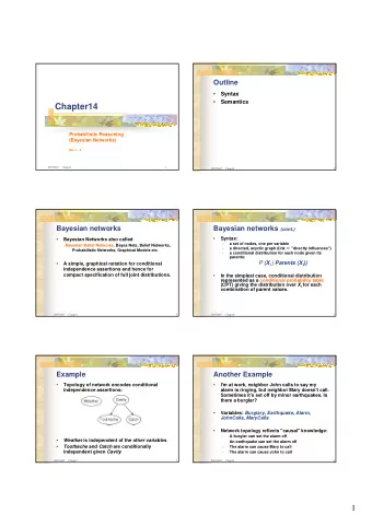
Bayesian networks A simple, graphical notation for conditional independence assertions and hence for compact specification of full joint distributions Syntax: – a set of nodes, one per variable – a directed, acyclic graph (link ≈ “directly influences”) – a conditional distribution for each node given its parents: P ( X i | Parents ( X i )) In the simplest case, the conditional distribution is represented as a conditional probability table (CPT) giving the distribution over X i for each combination of parent values of; based on AIMA Slides c Artificial Intelligence, spring 2013, Peter Ljungl¨ � Stuart Russel and Peter Norvig, 2004 Chapter 14, Sections 1–4 2
Example The topology of a network encodes conditional independence assertions: Cavity Weather Toothache Catch Weather is independent of the other variables Toothache and Catch are conditionally independent given Cavity of; based on AIMA Slides c Artificial Intelligence, spring 2013, Peter Ljungl¨ � Stuart Russel and Peter Norvig, 2004 Chapter 14, Sections 1–4 3
Example I’m at work. My neighbor John calls to say my alarm is ringing, but my neighbor Mary doesn’t call. Sometimes it’s set off by minor earthquakes. Is there a burglar? Variables: Burglar , Earthquake , Alarm , JohnCalls , MaryCalls The network topology reflects our “causal” knowledge: – a burglar can trigger the alarm – an earthquake can trigger the alarm – the alarm can cause Mary to call – the alarm can cause John to call of; based on AIMA Slides c Artificial Intelligence, spring 2013, Peter Ljungl¨ � Stuart Russel and Peter Norvig, 2004 Chapter 14, Sections 1–4 4
Example contd. P(E) P(B) Burglary Earthquake .002 .001 B E P(A|B,E) T T .95 Alarm T F .94 F T .29 F F .001 A P(J|A) A P(M|A) T .90 JohnCalls .70 MaryCalls T F .05 .01 F of; based on AIMA Slides c Artificial Intelligence, spring 2013, Peter Ljungl¨ � Stuart Russel and Peter Norvig, 2004 Chapter 14, Sections 1–4 5
Compactness A CPT for Boolean X i with k Boolean parents has B E 2 k rows for the combinations of parent values A Each row requires one number p for X i = true (the number for X i = false is just 1 − p ) J M If each variable has no more than k parents, the complete network requires O ( n · 2 k ) numbers I.e., it grows linearly with n , vs. O (2 n ) for the full joint distribution For the burglary net, 1 + 1 + 4 + 2 + 2 = 10 numbers (vs. 2 5 − 1 = 31 ) of; based on AIMA Slides c Artificial Intelligence, spring 2013, Peter Ljungl¨ � Stuart Russel and Peter Norvig, 2004 Chapter 14, Sections 1–4 6
Global semantics The global semantics defines the full joint distribution B E as the product of the local conditional distributions: A P ( x 1 , . . . , x n ) = Π n i = 1 P ( x i | parents ( X i )) J M e.g., P ( j ∧ m ∧ a ∧ ¬ b ∧ ¬ e ) = P ( j | a ) P ( m | a ) P ( a |¬ b, ¬ e ) P ( ¬ b ) P ( ¬ e ) = 0 . 9 × 0 . 7 × 0 . 001 × 0 . 999 × 0 . 998 ≈ 0 . 00063 of; based on AIMA Slides c Artificial Intelligence, spring 2013, Peter Ljungl¨ � Stuart Russel and Peter Norvig, 2004 Chapter 14, Sections 1–4 7
Markov blanket Theorem : Each node is conditionally independent of all others given its Markov blanket: parents + children + children’s parents U 1 U m . . . X Z 1j Z nj Y Y n 1 . . . of; based on AIMA Slides c Artificial Intelligence, spring 2013, Peter Ljungl¨ � Stuart Russel and Peter Norvig, 2004 Chapter 14, Sections 1–4 8
Constructing Bayesian networks We need a method such that a series of locally testable assertions of conditional independence guarantees the required global semantics 1. Choose an ordering of variables X 1 , . . . , X n 2. For i = 1 to n add X i to the network select parents from X 1 , . . . , X i − 1 such that P ( X i | Parents ( X i )) = P ( X i | X 1 , . . . , X i − 1 ) This choice of parents guarantees the global semantics: P ( X 1 , . . . , X n ) = Π n i = 1 P ( X i | X 1 , . . . , X i − 1 ) (chain rule) = Π n i = 1 P ( X i | Parents ( X i )) (by construction) of; based on AIMA Slides c Artificial Intelligence, spring 2013, Peter Ljungl¨ � Stuart Russel and Peter Norvig, 2004 Chapter 14, Sections 1–4 9
Example Suppose we choose the ordering M , J , A , B , E MaryCalls JohnCalls P ( J | M ) = P ( J ) ? of; based on AIMA Slides c Artificial Intelligence, spring 2013, Peter Ljungl¨ � Stuart Russel and Peter Norvig, 2004 Chapter 14, Sections 1–4 10
Example Suppose we choose the ordering M , J , A , B , E MaryCalls JohnCalls Alarm P ( J | M ) = P ( J ) ? No P ( A | J, M ) = P ( A | J ) ? P ( A | J, M ) = P ( A ) ? of; based on AIMA Slides c Artificial Intelligence, spring 2013, Peter Ljungl¨ � Stuart Russel and Peter Norvig, 2004 Chapter 14, Sections 1–4 11
Example Suppose we choose the ordering M , J , A , B , E MaryCalls JohnCalls Alarm Burglary P ( J | M ) = P ( J ) ? No P ( A | J, M ) = P ( A | J ) ? P ( A | J, M ) = P ( A ) ? No P ( B | A, J, M ) = P ( B | A ) ? P ( B | A, J, M ) = P ( B ) ? of; based on AIMA Slides c Artificial Intelligence, spring 2013, Peter Ljungl¨ � Stuart Russel and Peter Norvig, 2004 Chapter 14, Sections 1–4 12
Example Suppose we choose the ordering M , J , A , B , E MaryCalls JohnCalls Alarm Burglary Earthquake P ( J | M ) = P ( J ) ? No P ( A | J, M ) = P ( A | J ) ? P ( A | J, M ) = P ( A ) ? No P ( B | A, J, M ) = P ( B | A ) ? Yes P ( B | A, J, M ) = P ( B ) ? No P ( E | B, A, J, M ) = P ( E | A ) ? P ( E | B, A, J, M ) = P ( E | A, B ) ? of; based on AIMA Slides c Artificial Intelligence, spring 2013, Peter Ljungl¨ � Stuart Russel and Peter Norvig, 2004 Chapter 14, Sections 1–4 13
Example Suppose we choose the ordering M , J , A , B , E MaryCalls JohnCalls Alarm Burglary Earthquake P ( J | M ) = P ( J ) ? No P ( A | J, M ) = P ( A | J ) ? P ( A | J, M ) = P ( A ) ? No P ( B | A, J, M ) = P ( B | A ) ? Yes P ( B | A, J, M ) = P ( B ) ? No P ( E | B, A, J, M ) = P ( E | A ) ? No P ( E | B, A, J, M ) = P ( E | A, B ) ? Yes of; based on AIMA Slides c Artificial Intelligence, spring 2013, Peter Ljungl¨ � Stuart Russel and Peter Norvig, 2004 Chapter 14, Sections 1–4 14
Example contd. MaryCalls JohnCalls Alarm Burglary Earthquake Network is less compact: 1 + 2 + 4 + 2 + 4 = 13 numbers needed Compare with the original burglary net: 1 + 1 + 4 + 2 + 2 = 10 numbers of; based on AIMA Slides c Artificial Intelligence, spring 2013, Peter Ljungl¨ � Stuart Russel and Peter Norvig, 2004 Chapter 14, Sections 1–4 15
Example contd. The chosen ordering of the variables can have a big impact on the size of the network! Network (b) has 2 5 − 1 = 31 numbers—exactly the same as the full joint distribution of; based on AIMA Slides c Artificial Intelligence, spring 2013, Peter Ljungl¨ � Stuart Russel and Peter Norvig, 2004 Chapter 14, Sections 1–4 16
Inference tasks Simple queries: compute posterior marginal P ( X i | E = e ) e.g., P ( Burglar | JohnCalls = true, MaryCalls = true ) or shorter, P ( B | j, m ) Conjunctive queries: P ( X i , X j | E = e ) = P ( X i | E = e ) P ( X j | X i , E = e ) Optimal decisions: decision networks include utility information; probabilistic inference required for P ( outcome | action, evidence ) Value of information: which evidence to seek next? Sensitivity analysis: which probability values are most critical? Explanation: why do I need a new starter motor? of; based on AIMA Slides c Artificial Intelligence, spring 2013, Peter Ljungl¨ � Stuart Russel and Peter Norvig, 2004 Chapter 14, Sections 1–4 17
Inference by enumeration Slightly intelligent way to sum out variables from the joint without actually constructing its explicit representation Simple query on the burglary network: B E P ( B | j, m ) = P ( B, j, m ) /P ( j, m ) A = α P ( B, j, m ) J M = α Σ e Σ a P ( B, e, a, j, m ) (where e and a are the hidden variables) Rewrite full joint entries using product of CPT entries: P ( B | j, m ) = α Σ e Σ a P ( B ) P ( e ) P ( a | B, e ) P ( j | a ) P ( m | a ) = α P ( B ) Σ e P ( e ) Σ a P ( a | B, e ) P ( j | a ) P ( m | a ) Recursive depth-first enumeration: O ( n ) space, O ( d n ) time of; based on AIMA Slides c Artificial Intelligence, spring 2013, Peter Ljungl¨ � Stuart Russel and Peter Norvig, 2004 Chapter 14, Sections 1–4 18
Evaluation tree P(b) .001 P(e) P( e) .002 .998 P( a|b, e) P(a|b,e) P( a|b,e) P(a|b, e) .95 .05 .94 .06 P(j|a) P(j| a) P(j|a) P(j| a) .90 .05 .90 .05 P(m|a) P(m| a) P(m|a) P(m| a) .70 .01 .70 .01 Enumeration is inefficient: repeated computation e.g., computes P ( j | a ) P ( m | a ) for each value of e of; based on AIMA Slides c Artificial Intelligence, spring 2013, Peter Ljungl¨ � Stuart Russel and Peter Norvig, 2004 Chapter 14, Sections 1–4 19
Recommend
More recommend
Explore More Topics
Stay informed with curated content and fresh updates.
