Lecture 14: Learning Theory (Part 3) March 2020 Lecturer: Steven Wu - PDF document

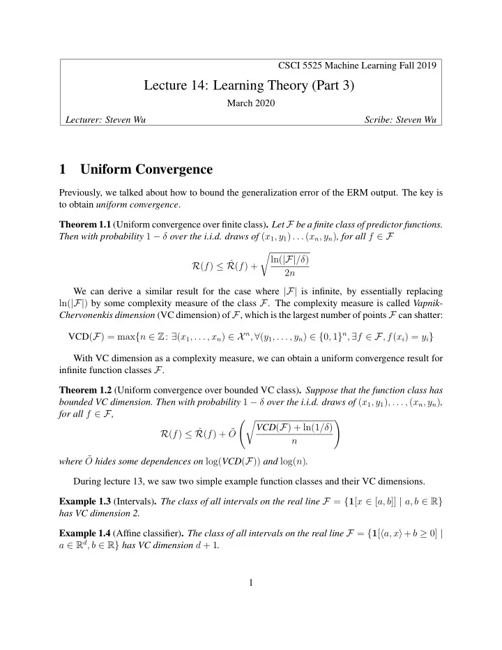
CSCI 5525 Machine Learning Fall 2019 Lecture 14: Learning Theory (Part 3) March 2020 Lecturer: Steven Wu Scribe: Steven Wu 1 Uniform Convergence Previously, we talked about how to bound the generalization error of the ERM output. The key is to obtain uniform convergence . Theorem 1.1 (Uniform convergence over finite class) . Let F be a finite class of predictor functions. Then with probability 1 − δ over the i.i.d. draws of ( x 1 , y 1 ) . . . ( x n , y n ) , for all f ∈ F � ln( |F| /δ ) R ( f ) ≤ ˆ R ( f ) + 2 n We can derive a similar result for the case where |F| is infinite, by essentially replacing ln( |F| ) by some complexity measure of the class F . The complexity measure is called Vapnik- Chervonenkis dimension (VC dimension) of F , which is the largest number of points F can shatter: VCD ( F ) = max { n ∈ Z : ∃ ( x 1 , . . . , x n ) ∈ X n , ∀ ( y 1 , . . . , y n ) ∈ { 0 , 1 } n , ∃ f ∈ F , f ( x i ) = y i } With VC dimension as a complexity measure, we can obtain a uniform convergence result for infinite function classes F . Theorem 1.2 (Uniform convergence over bounded VC class) . Suppose that the function class has bounded VC dimension. Then with probability 1 − δ over the i.i.d. draws of ( x 1 , y 1 ) , . . . , ( x n , y n ) , for all f ∈ F , �� � VCD ( F ) + ln(1 /δ ) R ( f ) ≤ ˆ R ( f ) + ˜ O n where ˜ O hides some dependences on log( VCD ( F )) and log( n ) . During lecture 13, we saw two simple example function classes and their VC dimensions. Example 1.3 (Intervals) . The class of all intervals on the real line F = { 1 [ x ∈ [ a, b ]] | a, b ∈ R } has VC dimension 2. Example 1.4 (Affine classifier) . The class of all intervals on the real line F = { 1 [ � a, x � + b ≥ 0] | a ∈ R d , b ∈ R } has VC dimension d + 1 . 1

We can also obtain VC dimension bound for neural networks, which depends on the choices of activation functions. Example 1.5 (Neural networks) . Consider the classifier given by neural networks: for each feature vector x , the prediction is given by f ( x, θ ) = sgn [ σ L ( W L ( . . . W 2 σ 1 ( W 1 x + b 1 ) + b 2 . . . ) + b L )] Let ρ be the number of parameters (weights and biases), L be the number of layers, and m be the number of nodes. If we use the same activation for all σ i , we can obtain: • Binary activation σ ( z ) = 1 [ z ≥ 0] , VCD = O ( ρ ln ρ ) . (See Theorem 4 of this paper for a proof.) • ReLU activation σ ( z ) = max(0 , z ) , VCD = O ( ρL ln( ρL )) (See Theorem 6 of this paper for a proof.) Roughly speaking, the VC-dimension of a neural network scales with the number of parameters defining class F . However, in practice, the number of parameters might exceed the number of training examples, so the generalization bound derived from VC dimension is often not very useful for deep nets. Here is a simple example for which the VC dimension is very different frorm the number of parameters. Consider, for example, the domain X = R , and the class F = { h θ : θ ∈ R where h θ : X → { 0 , 1 } is defined by h θ ( x ) = ⌈ 0 . 5 sin( θx ) ⌉ . It is possible to prove that VCD ( F ) = ∞ . 2 Rademacher Complexity Well, VC dimension is designed for binary classification. How about other learning problems including multi-class classification and regression? There is actually a more general complexity measure. Given a set of examples S = { z 1 . . . , z n } and function class F , the Rademacher complexity is defined as n 1 � Rad ( F , S ) = E ǫ sup ǫ i f ( z i ) n f ∈F i =1 where each ǫ 1 , . . . , ǫ n are i.i.d. Rademacher random variables: Pr [ ǫ i = 1] = Pr [ ǫ i = − 1] = 1 / 2 . Why does Rademacher complexity capture the complexity of a function class? One intuition is that it captures the ability of F to fit random signs given by the Rademacher random variables. For any loss function ℓ : Y × Y and predictor f ∈ F , let ℓ ◦ f be a function such that for any example z = ( x, y ) ℓ ◦ f ( z ) = ℓ ( y, f ( x )) Let the corresponding function class ℓ ◦ F = { ℓ ◦ f | f ∈ F} . Now we can derive the following generalization bound using Rademacher complexity. 2

Theorem 2.1. Assume that for all z = ( x, y ) ∈ X × Y and f ∈ F we have | ℓ ( y, f ( x ) | ≤ c . Let z 1 = ( x 1 , y 1 ) , . . . , z n = ( x n , y n ) be i.i.d. draws from the underlying distribution P . Then with probability at least 1 − δ , for all f ∈ F � 2 ln(4 /δ ) R ( f ) ≤ ˆ R ( f ) + 2 Rad ( ℓ ◦ F , S ) + 4 c n Moreover, if ℓ is γ -Lipschitz in the second argument for all y , then Rad ( ℓ ◦ F , S ) ≤ γ Rad ( F , S ) , and so � 2 ln(4 /δ ) R ( f ) ≤ ˆ R ( f ) + 2 γ Rad ( F , S ) + 4 c n Note that Rademacher complexity depends on the underlying data distribution. For simple function classes, we can obtain complexity bounds only by assuming boundedness in the data. Example 2.2 (Linear predictors) . Consider two classes of linear functions: F 1 = { x → w ⊺ x : w ∈ R d , � w � 1 ≤ W 1 } F 2 = { x → w ⊺ x : w ∈ R d , � w � 2 ≤ W 2 } Let S = ( x 1 , ..., x n ) be vectors in R d . � 2 log(2 d ) Rad ( F 1 , S ) ≤ (max � x i � ∞ ) W 1 n i � 1 Rad ( F 2 , S ) ≤ (max � x i � 2 ) W 2 n i For linear functions, a nice feature of Rademacher complexity is that it picks up explicit depen- dence on the norm bounds of the weight vectors. In comparison, the VC dimension for the class of affine functions is just d + 1 . 3