Duality Marco Chiarandini Department of Mathematics & Computer - PowerPoint PPT Presentation
DM545/DM554 Linear and Integer Programming Lecture 5 Duality Marco Chiarandini Department of Mathematics & Computer Science University of Southern Denmark Derivation and Motivation Outline Theory 1. Derivation and Motivation 2. Theory
DM545/DM554 Linear and Integer Programming Lecture 5 Duality Marco Chiarandini Department of Mathematics & Computer Science University of Southern Denmark
Derivation and Motivation Outline Theory 1. Derivation and Motivation 2. Theory 2
Derivation and Motivation Outline Theory 1. Derivation and Motivation 2. Theory 3
Derivation and Motivation Dual Problem Theory Dual variables y in one-to-one correspondence with the constraints: Primal problem: Dual Problem: w = b T y min z = c T x max A T y ≥ c A x ≤ b y ≥ 0 x ≥ 0 4
Derivation and Motivation Bounding approach Theory z ∗ = max 4 x 1 + x 2 + 3 x 3 x 1 + 4 x 2 ≤ 1 3 x 1 + x 2 + x 3 ≤ 3 x 1 , x 2 , x 3 ≥ 0 a feasible solution is a lower bound but how good? By tentatives: ( x 1 , x 2 , x 3 ) = ( 1 , 0 , 0 ) � z ∗ ≥ 4 ( x 1 , x 2 , x 3 ) = ( 0 , 0 , 3 ) � z ∗ ≥ 9 What about upper bounds? 2 · ( x 1 + 4 x 2 ) ≤ 2 · 1 + 3 · ( 3 x 1 + x 2 + x 3 ) ≤ 3 · 3 4 x 1 + x 2 + 3 x 3 ≤ 11 x 1 + 11 x 2 + 3 x 3 ≤ 11 c T x y T Ax ≤ y T b ≤ Hence z ∗ ≤ 11. Is this the best upper bound we can find? 5
Derivation and Motivation Theory multipliers y 1 , y 2 ≥ 0 that preserve sign of inequality y 1 · ( x 1 + 4 x 2 ) ≤ y 1 ( 1 ) y 2 · ( 3 x 1 + x 2 + x 3 ) ≤ y 2 ( 3 ) ( y 1 + 3 y 2 ) x 1 + ( 4 y 1 + y 2 ) x 2 + y 2 x 3 ≤ y 1 + 3 y 2 Coefficients y 1 + 3 y 2 ≥ 4 4 y 1 + y 2 ≥ 1 y 2 ≥ 3 z = 4 x 1 + x 2 + 3 x 3 ≤ ( y 1 + 3 y 2 ) x 1 + ( 4 y 1 + y 2 ) x 2 + y 2 x 3 ≤ y 1 + 3 y 2 then to attain the best upper bound: min y 1 + 3 y 2 y 1 + 3 y 2 ≥ 4 4 y 1 + y 2 ≥ 1 y 2 ≥ 3 y 1 , y 2 ≥ 0 6
Derivation and Motivation Multipliers Approach Theory a 11 a 12 . . . a 1 n a 1 , n + 1 a 1 , n + 2 . . . a 1 , m + n 0 b 1 π 1 . . ... . . . . a m 1 a m 2 . . . a mn a m , n + 1 a m , n + 2 . . . a m , m + n 0 b m π m 0 0 0 1 0 c 1 c 2 . . . c n π m + 1 . . . Working columnwise, since at optimum ¯ c k ≤ 0 for all k = 1 , . . . , n + m : π 1 a 11 + π 2 a 21 . . . + π m a m 1 + π m + 1 c 1 ≤ 0 . . ... . . . . + . . . + + π m + 1 c n ≤ 0 π 1 a 1 n π 2 a 2 n π m a mn π 1 a 1 , n + 1 , π 2 a 2 , n + 1 , . . . π m a m , n + 1 ≤ 0 . . . . . . . . . . . . . . . . . . π 1 a 1 , n + m , π 2 a 2 , n + m , . . . π m a m , n + m ≤ 0 = 1 π m + 1 π 1 b 1 + π 2 b 2 . . . + π m b m ( ≤ 0 ) (since from the last row z = − π π b and we want to maximize z then we would min ( − π π b ) or π π equivalently max π π b ) π 7
Derivation and Motivation Theory max π 1 b 1 + π 2 b 2 . . . + π m b m π 1 a 11 + π 2 a 21 . . . + π m a m 1 ≤ − c 1 . . ... . . . . π 1 a 1 n + π 2 a 2 n . . . + π m a mn ≤ − c n 0 π 1 , π 2 , . . . π m ≤ y = − π max − y 1 b 1 + − y 2 b 2 . . . + − y m b m − y 1 a 11 + − y 2 a 21 . . . + − y m a m 1 ≤ − c 1 . . ... . . . . − y 1 a 1 n + − y 2 a 2 n . . . + − y m a mn ≤ − c n − y 1 , − y 2 , . . . − y m ≤ 0 w = b T y min A T y ≥ c y ≥ 0 8
Derivation and Motivation Example Theory max 6 x 1 + 8 x 2 5 x 1 + 10 x 2 ≤ 60 4 x 1 + 4 x 2 ≤ 40 x 1 , x 2 ≥ 0 5 π 1 + 4 π 2 + 6 π 3 ≤ 0 10 π 1 + 4 π 2 + 8 π 3 ≤ 0 1 π 1 + 0 π 2 + 0 π 3 ≤ 0 0 π 1 + 1 π 2 + 0 π 3 ≤ 0 0 π 1 + 0 π 2 + 1 π 3 = 1 60 π 1 + 40 π 2 y 1 = − π 1 ≥ 0 y 2 = − π 2 ≥ 0 ... 9
Derivation and Motivation Duality Recipe Theory 10
Derivation and Motivation Outline Theory 1. Derivation and Motivation 2. Theory 11
Derivation and Motivation Symmetry Theory The dual of the dual is the primal: Primal problem: Dual Problem: w = b T y min z = c T x max A T y ≥ c Ax ≤ b y ≥ 0 x ≥ 0 Let’s put the dual in the standard form Dual problem: Dual of Dual: − min − c T x min b T y ≡ − max − b T y − Ax ≥ − b − A T y ≤ − c ≥ 0 x ≥ 0 y 12
Derivation and Motivation Weak Duality Theorem Theory As we saw the dual produces upper bounds. This is true in general: Theorem (Weak Duality Theorem) Given: (P) max { c T x | A x ≤ b , x ≥ 0 } (D) min { b T y | A T y ≥ c , y ≥ 0 } for any feasible solution x of (P) and any feasible solution y of (D): c T x ≤ b T y Proof: From (D) c j ≤ � m i = 1 y i a ij ∀ j and from (P) � n j = 1 a ij x i ≤ b i ∀ i From (D) y i ≥ 0 and from (P) x j ≥ 0 � � n n m m n m � � � � � � y i ≤ c j x j ≤ y i a ij x j = a ij x i b i y i j = 1 j = 1 i = 1 i = 1 j = 1 i = 1 13
Derivation and Motivation Strong Duality Theorem Theory Due to Von Neumann and Dantzig 1947 and Gale, Kuhn and Tucker 1951. Theorem (Strong Duality Theorem) Given: (P) max { c T x | Ax ≤ b , x ≥ 0 } (D) min { b T y | A T y ≥ c , y ≥ 0 } exactly one of the following occurs: 1. (P) and (D) are both infeasible 2. (P) is unbounded and (D) is infeasible 3. (P) is infeasible and (D) is unbounded 4. (P) has feasible solution x ∗ = [ x ∗ 1 , . . . , x ∗ n ] (D) has feasible solution y ∗ = [ y ∗ 1 , . . . , y ∗ m ] c T x ∗ = b T y ∗ 14
Derivation and Motivation Theory Proof: • all other combinations of 3 possibilities (Optimal, Infeasible, Unbounded) for (P) and 3 for (D) are ruled out by weak duality theorem. • we use the simplex method. (Other proofs independent of the simplex method exist, eg, Farkas Lemma and convex polyhedral analysis) • The last row of the final tableau will give us n + m n m � � � z = z ∗ + c k x k = z ∗ + ¯ ¯ c j x j + ¯ (*) c n + i x n + i k = 1 j = 1 i = 1 = z ∗ + ¯ c B x B + ¯ c N x N In addition, z ∗ = � n j = 1 c j x ∗ j because optimal value • We define y ∗ i = − ¯ c n + i , i = 1 , 2 , . . . , m m ) is a dual feasible solution satisfying c T x ∗ = b T y ∗ . • We claim that ( y ∗ 1 , y ∗ 2 , . . . , y ∗ 15
Derivation and Motivation Theory • Let’s verify the claim: We substitute in (*): i) z = � n i ; and iii) x n + i = b i − � n c n + i = − y ∗ j = 1 c j x j ; ii) ¯ j = 1 a ij x j for i = 1 , 2 , . . . , m ( n + i are the slack variables) n n m n � � � � c j x j = z ∗ + y ∗ c j x j − ¯ b i − a ij x j i j = 1 j = 1 i = 1 j = 1 � � � � m n m � � � z ∗ − y ∗ a ij y ∗ = i b i + c j + ¯ x j i i = 1 j = 1 i = 1 This must hold for every ( x 1 , x 2 , . . . , x n ) hence: m � z ∗ = ⇒ y ∗ satisfies c T x ∗ = b T y ∗ b i y ∗ = i i = 1 m � a ij y ∗ c j = ¯ c j + i , j = 1 , 2 , . . . , n i = 1 16
Derivation and Motivation Theory Since ¯ c k ≤ 0 for every k = 1 , 2 , . . . , n + m : m m � � y ∗ y ∗ c j ≤ 0 � ¯ c j − i a ij ≤ 0 � i a ij ≥ c j j = 1 , 2 , . . . , n i = 1 i = 1 y ∗ c n + i ≤ 0 � ¯ i = − ¯ c n + i ≥ 0 , i = 1 , 2 , . . . , m ⇒ y ∗ is also dual feasible solution = 17
Derivation and Motivation Complementary Slackness Theorem Theory Theorem (Complementary Slackness) A feasible solution x ∗ for (P) A feasible solution y ∗ for (D) Necessary and sufficient conditions for optimality of both: � � m � y ∗ x ∗ c j − j = 0 , j = 1 , . . . , n i a ij i = 1 j � = 0 then � y ∗ If x ∗ i a ij = c j (no surplus) If � y ∗ i a ij > c j then x ∗ j = 0 Proof: In scalars z ∗ = c T x ∗ ≤ y ∗ A x ∗ ≤ b T y ∗ = w ∗ n m � � y ∗ ) x ∗ ( c j − = 0 i a ij j ���� j = 1 i = 1 Hence from strong duality theorem: ≥ 0 � �� � ≤ 0 cx ∗ − y ∗ A x ∗ = 0 Hence each term must be = 0 18
Derivation and Motivation Theory Proof in scalar form: � m � � c j x ∗ a ij y ∗ x ∗ j ≤ j = 1 , 2 , . . . , n from feasibility in D i j i = 1 n � a ij x ∗ y ∗ i ≤ b i y ∗ i = 1 , 2 , . . . , m from feasibility in P j i j = 1 Summing in j and in i : � m � n n m n m � � � � � � c j x ∗ a ij y ∗ x ∗ a ij x ∗ y ∗ b i y ∗ j ≤ j = i ≤ i j i j = 1 j = 1 i = 1 i = 1 j = 1 i = 1 For the strong duality theorem the left hand side is equal to the right hand side and hence all inequalities become equalities. n m � � y ∗ ) x ∗ ( c j − = 0 i a ij j ���� j = 1 i = 1 ≥ 0 � �� � ≤ 0 19
Derivation and Motivation Duality - Summary Theory • Derivation: • Economic interpretation • Bounding Approach • Multiplier Approach • Recipe • Lagrangian Multipliers Approach (next time) • Theory: • Symmetry • Weak Duality Theorem • Strong Duality Theorem • Complementary Slackness Theorem 20
Recommend
More recommend
Explore More Topics
Stay informed with curated content and fresh updates.
