Lecture 13 : The Exponential Distribution 0/ 19 Definition A - PDF document
Lecture 13 : The Exponential Distribution 0/ 19 Definition A continuous random variable X is said to have exponential distribution with parameter . If the pdf of X is (with > 0 ) e x , x > 0 f ( x ) = (*) 0 ,
Lecture 13 : The Exponential Distribution 0/ 19
Definition A continuous random variable X is said to have exponential distribution with parameter λ . If the pdf of X is (with λ > 0 ) � λ e − λ x , x > 0 f ( x ) = (*) 0 , otherwise Remarks Very often the independent variable will be time t rather than x. The exponential distribution is the special case of the gamma distribution with α = 1 and β = 1 α . We will see that X β closely tied to the Poisson process, that is why λ is used above. 1/ 19 Lecture 13 : The Exponential Distribution
Here is the graph of f 1 Proposition ((cdf) (Prove this)) If X has exponential distribution then F ( x ) = P ( X ≤ x ) = 1 − e − λ x Corollary (Prove this) If X has exponential distribution P ( X > x ) = e − λ x This is a very useful formula. 2/ 19 Lecture 13 : The Exponential Distribution
Proposition If X has exponential distribution (i) E ( X ) = 1 λ (ii) V ( X ) = 1 λ 2 The Physical Meaning of the Exponential Distribution Recall (Lecture 8) that the binomial process (having a a child, flipping a coin) gave rise to two (actually infinitely many) more distributions 1 X = the geometric distribution = the waiting time for the first girl 3/ 19 Lecture 13 : The Exponential Distribution
and X r = the negative binomial = the waiting time for the r -th girl Remark Here time was discrete. Also X r was the number of boys before the r-th girl so the waiting time was actually Y r = X r + r − 1 . Now we will see the same thing happens with a Poisson process. Now time is continuous, as I warned you. I will switch from x to t in (*). 4/ 19 Lecture 13 : The Exponential Distribution
So suppose we have a trap to catch some species of animal. We run it forever starting at time t = 0, so 0 ≤ t < ∞ . The Counting Random Variable Now fix a time period t . So we have a “counting random variable X t ”. X t = ♯ of animals caught in the trap in time t . We will choose the model X t ∼ P ( λ t ) = Poisson with parameter λ t . Z We are using λ instead of α in the Poisson process N.B. P ( X t = 0 ) = e − λ t ( ♯ ) 5/ 19 Lecture 13 : The Exponential Distribution
Remark The analogue from before was X n = ♯ of girls in the first n children (so we have a discrete “time period”, the binomial random variable was the counting random variable.) Now we want to consider the analogue of the “waiting time” random variables, the geometric and negative binomials for the binomial process. Let Y = the time when the first animal is caught. 6/ 19 Lecture 13 : The Exponential Distribution
The proof of the following theorem involves such a beautiful simple idea I am going to give it. Theorem Y has exponential distribution with parameter α . Proof We will compute P ( Y > t ) and show P ( Y > t ) = e − λ t ( so F ( t ) = P ( Y ≤ t ) = 1 − e − λ t and f ( t ) = F ′ ( λ ) = λ e − λ t ) 7/ 19 Lecture 13 : The Exponential Distribution
Proof (Cont.) Here is the beautiful observation. You have to wait longer than t units for the first animal to be caught ⇔ there are no animals in the trap at time t. In symbols this says equality of events But we have seen P ( X t = 0 ) = e − λ t so necessarily P ( Y > t ) = e − λ t � 8/ 19 Lecture 13 : The Exponential Distribution
Now what about the analogue of the negative binomial = the waiting time for the n -th girl. The r -Erlang Distribution Let Y r = the waiting until the r -th animal is caught. Theorem (i) The cdf F r of Y r is given by + · · · + ( λ t ) r − 1 1 − ( 1 + λ + ( λ t ) 2 ( r − 1 )! , e − λ t , t > 0 2 ! F r ( t ) = 0 , otherwise (ii) Differentiating (this is tricky) F r ( t ) to get the pdf f r ( t ) we get λ r t r − 1 ( r − 1 )! e − λ t , t > 0 f r ( t ) = 0 , otherwise Remark This distribution is called the r-Erlang distribution. 9/ 19 Lecture 13 : The Exponential Distribution
Proof We use the same trick as before P ( Y r > t ) = P ( X t ≤ r − 1 ) The waiting time for the r-th animal to arrive in the trap is > t ⇔ at time t there are ≤ r − 1 animals in the trap. Since X t ∼ P ( λ t ) we have P ( X t ≤ r − 1 ) = e − λ t + e − λ t λ t + e − λ t ( λ t ) 2 2 ! + · · · + e − λ t ( λ t ) r − 1 ( r − 1 )! 10/ 19 Lecture 13 : The Exponential Distribution
Proof (Cont.) Now we have to do some hard computation. 1 + λ t + · · · + ( λ t ) r − 1 � � P ( X t ≤ r − 1 ) = e − λ t ( r − 1 )! So F r ( t ) = P ( Y r ≤ t ) = 1 − P ( Y r > t ) 1 + λ t + · · · + ( λ t ) r − 1 � � = 1 − e − λ t ( r − 1 )! f r ( t ) = dF r dt ( t ) But So we have to differentiate the expression on the right-hand side d Of course dt ( 1 ) = 0 11/ 19 Lecture 13 : The Exponential Distribution
Proof (Cont.) A hard derivative computation 1 + λ t + ( λ t ) 2 + · · · + ( λ t ) r − 2 ( r − 2 !) + ( λ t ) r − ? f r ( t ) = −− d � � dt ( e − λ t ) 2 ! ( r − 1 )! 1 + λ t + ( λ t ) 2 + · · · + ( λ t ) r − 1 � � − e − λ t d 1 ! ( r − 1 )? dt 1 + λ t + ( λ t ) 2 + · · · + ( λ t ) r − 2 ( r − 2 )! + ( λ t ) r − 1 � � = λ e − λ t 2 ! ( r − 1 )! λ + λ 2 t + λ 3 t 2 2 ! + · · · + λ r − 1 t r − 2 � � − e − λ t ( r − 2 )! ✚✚✚✚ ✚ � λ 3 t 2 λ r − 1 t r − 2 ( r − 2 )! + λ r t r − 1 λ 2 + + � � = e − λ t ✁ λ + � 2 ! + · · · + � ( r − 1 )! � � � � ✚✚✚✚ ✚ � λ 2 t 2 λ r − 1 t r − 2 λ 2 + + � � − e − λ t ✁ λ + � 2 ! + · · · + � ( r − 2 )! = λ r t r − 1 ( r − 1 )! e − λ t � 12/ 19 Lecture 13 : The Exponential Distribution
Lifetimes and Failure Times for Components and Systems Suppose each of the components has a lifetime that is exponentially distributed with parameter λ (see below for a more precise statement). Assume the components are independent. How is the system lifetime distributed? 13/ 19 Lecture 13 : The Exponential Distribution
Solution Define random variables X 1 , X 2 , X 3 by ( X i = t ) = ( C i fails at time t ) , i = 1 , 2 , 3 Then X i is exponentially distributed with parameter λ so P ( X i ≤ t ) = 1 − e − λ t , i = 1 , 2 , 3 P ( X i > t ) = e − λ , i = 1 , 2 , 3 . Define Y by ( Y = t ) = ( system fails at time t ) 14/ 19 Lecture 13 : The Exponential Distribution
Solution (Cont.) The key step (using the geometry of the system) Lump C 1 and C 2 into a single component A and let W be the corresponding random variable so ( W = t ) = ( A fails at time t ) ( Y > t ) = ( W > t ) ∩ ( X 3 > t ) (the system is working at time t ⇔ both A and C 3 are working at time t) 15/ 19 Lecture 13 : The Exponential Distribution
The Golden Rule Try to get ∩ instead of ∪ - that’s why I choose ( Y > t ) on the left. Hence P ( Y > t ) = P (( W > t ) ∩ ( X 3 > t )) by independence = P ( W > t ) · P ( X 3 > t ) ( ♯ ) Why are ( W > t ) and ( X 3 > t ) independent? Answer Suppose C 1 , C 2 , . . . C n are independent components. Suppose A = a subcollection of the C i ’s. B = another subcollection of the C i ’s. 16/ 19 Lecture 13 : The Exponential Distribution
Answer (Cont.) Then A and B are independent ⇔ they have no common component. So now we need P ( W > t ) where W is I should switch to P ( W ≤ t ) to get intersections but I won’t to show you why unions give extra terms. 17/ 19 Lecture 13 : The Exponential Distribution
( W > t ) = ( X 1 > t ) ∪ ( X 2 > t ) ( A is working at time t ⇔ either C 1 is or C 2 is) So extra term 18/ 19 Lecture 13 : The Exponential Distribution
Now from ( ♯ ) P ( Y > t ) = P ( W > t ) P ( X 3 > t ) = ( 2 e − λ t − e − 2 λ t ) e − λ t P ( Y > t ) = 2 e − 2 λ t − e − 3 λ t so the cdf of Y is given by P ( Y ≤ t ) = 1 − P ( Y > t ) = 1 − 2 e − 2 λ t + e − 3 λ t That’s good enough. 19/ 19 Lecture 13 : The Exponential Distribution
Recommend
More recommend
Explore More Topics
Stay informed with curated content and fresh updates.
