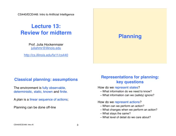
Lecture 13: Review for midterm Planning Prof. Julia Hockenmaier - PowerPoint PPT Presentation

CS440/ECE448: Intro to Artificial Intelligence � Lecture 13: 
 Review for midterm � Planning � Prof. Julia Hockenmaier � juliahmr@illinois.edu � � http://cs.illinois.edu/fa11/cs440 � � � Representations for planning: 
 Classical planning: assumptions � key questions � How do we represent states? � The environment is fully observable, 
 – What information do we need to know? � deterministic, static, known and finite. � – What information can we (safely) ignore? � � � A plan is a linear sequence of actions; � How do we represent actions? � � – When can we perform an action? � Planning can be done off-line � – What changes when we perform an action? � – What stays the same? � – What level of detail do we care about? � CS440/ECE448: Intro AI � 3 �

Representations for operators � Operators, actions and fluents � Operator : carry(x) 
 Operator name (and arity): move x from y to z � General knowledge of one kind of action: 
 � � move(x,y,z) preconditions and effects � � Preconditions: when can the action be performed � Action : carry(BlockA) 
 clear(x) ∧ clear(z) ∧ on(x,y) Ground instance of an operator � � Fluent : on(BlockA, BlockB, s) Effects : how does the world change? � may be true in current state, but not after the clear(y) ∧ on(x,z) ∧ clear(x) ∧ ¬clear(z) ∧ ¬on(x,y) action move(A,B,T) is performed. � new persist retract => main differences between languages � � � CS440/ECE448: Intro AI � 6 � Representations for states � Representations for planning � Situation Calculus � Strips � We want to know what state the world is in: � Specify fluents 
 Specify fluents � – What are the current properties of the entities? � Add -set 
 Add -set � – What are the current relations between the Persist -set � Delete -set � entities? � � � By default fluents 
 By default fluents persist � Logic representation: � are deleted � Each state is a conjunction of ground predicates: � Block(A) ∧ Block(B) ∧ Block(C) ∧ Table(T) ∧ On(A,B) ∧ On(B,T) ∧ On(C,T) ∧ Clear(A) ∧ Clear(C)

Planning algorithms � Planning as state space search � Search tree: � State space search (DFS, BFS, etc.) � – Nodes: states � Nodes = states; edges = actions; � – Root: initial state � Heuristics (make search more efficient) � – Edges: actions (ground instances of operators � Compute h() using relaxed version of the problem � Plan space search (refinement of partial plans) � – Solutions: paths from initial state to goal. � Nodes = partial plans; edges: fix flaws in plan � I,a4 � SATplan (encode plan in propositional logic) � I,a2 � I,a4,a3 � I � Solution = true variables in a model for the plan � I,a2,a34 � Graphplan (reduce search space to planning graph) � I,a15 � Planning graph: levels = literals and actions � I,a15,a4 � I,a17 � CS440/ECE448: Intro AI � 9 � Searching plan-space � SATplan � 1. Start with the empty plan 
 Represent a plan of fixed length n 
 = {start state, goal state} as a ground formula in predicate logic. � � Translate this formula into propositional logic. � 2. Iteratively refine current plan to resolve flaws 
 � � (refine = add new actions and constraints) � There is a solution if this formula is satisfiable. � – Flaw type 1: open goals (require more actions) � Plan = sequence of ʻ true ʼ actions. � – Flaw type 2: threats (require ordering constraints) � � � If there is no solution of length n, try n+1. � 3. Solution = a plan without flaws � � CS440/ECE448: Intro AI � 11 � CS440/ECE448: Intro AI � 12 �


 From plans to predicate logic � From plans to propositional logic � Fluents are ground literals: clear(B, t) � Fluents 
 clear(B, 23) = clear-B-23 � Actions are ground implications: 
 ( preconditions t ∧ action t ) ! effect t+1 Actions 
 ( (on(A,B, 23) ∧ clear(C,23) ∧ move(A,B,C, 23) ) Action move(A,B,C, 23) ! (on(A,C, 24) ∧ clear(B, 24)) ( on(A,B, 23) ∧ clr(C, 23) ∧ move(A,B,C, 23) ) ((on-A-B-23 ∧ clear-C-23) ∧ move-A-B-C-23)) ! (on(A,C, 24) ∧ clr(B, 24)) ! (on-A-C-24 ∧ clear-B-24) CS440/ECE448: Intro AI � 13 � CS440/ECE448: Intro AI � 14 � Key concepts � Agents: � – Different kinds of agents � – The structure and components of agents 
 � Intelligent agents � Describing and evaluating agents: � – Performance measures � – Task environments 
 � Rationality: � – What makes an agent intelligent? � �


 
 Agents � Task environments � 1. What is the task environment of: � The task environment specifies the problem that the agent has to solve. � – a chess computer? � � – a Mars rover? � It is defined by: � – a spam detector? � 1. the objective P erformance measure � � 2. the external E nvironment � 2. What is the advantage of model-based 3. the agent ʼ s A ctuators � agents over reflex-based agents? � 4. the agent ʼ s S ensors � � CS440/ECE448: Intro AI � 18 � � Simple reflex agents � Model-based reflex agents � Action depends only on current percept. � Agent has an internal model 
 Agent has no memory. 
 of the current state of the world. � Examples: the agent ʼ s previous location; current Last percept � Action � locations of all objects it has seen; 
 [Clean] � Right � � � [ cat ] � RUN! � Last percept � Last location � Action � May choose actions stochastically 
 [Clean] � Left of current � Right � to escape infinite loops. � [Clean] � Right of current � Left � � Last percept � Action � � [Clean] � Right (p=0.8) Left(p=0.2) � � CS440/ECE448: Intro AI � 19 � CS440/ECE448: Intro AI � 20 �


 Key concepts � Problem solving as search: � Solution = a finite sequence of actions 
 � State graphs and search trees � Systematic search � Which one is bigger/better to search? 
 � Systematic (blind) search algorithms � Breadth-first vs. depth-first; properties? 
 � � � CS440/ECE448: Intro AI � 22 � Systematic/blind search: The queuing function defines 
 assumptions � the search order � Depth-first search � (LIFO) �� The environment is: � A Expand deepest node first � 1. observable 
 B C D (Agent perceives all it needs to know) � QF(old, new): 
 2. known 
 � Append(new, old) 
 E F G H I � J (Agent knows the effects of each action) � � 3. deterministic 
 A Breadth-first (FIFO) � (Each action always has the same outcome) 
 Expand nodes level by level � B C D � In such environments, the solution to any QF(old, new): 
 E F G H I � J problem is a fixed sequence of actions. � � Append(old, new); � �

State-space graph � Solution � Goal � Goal � state � state � Initial � Initial � b3 � c5 � b3 � c5 � state � state � ! ! a1 � a1 � …. …. "! "! ! ! ! ! ! ! b4 � b4 � ! "! "! "! ! "! "! "! "! "! a2 � a2 � ! ! a3 � a3 � "! "! b1 � b1 � ! ! "! "! Nodes : states � A single path ! ! b2 � b2 � "! ! "! ! Edges: actions � from the initial "! "! Edge weights: state to a goal ! ! "! "! cost of actions � state. � ! ! ! ! "! "! …. …. "! "! …. …. Goal � Goal � Goal � Goal � ! ! ! ! state � state � state � state � "! "! "! "! Properties of search algorithms � A search algorithm is complete 
 if it will find any goal whenever one exists. � Informed (heuristic) A search algorithm is optimal 
 if it will find the cheapest goal. � search � Time complexity: how long does it take to find a solution? � Space complexity: how much memory does it take to find a solution? � � 27 �


 
 Informed search: 
 Heuristic search: priority queue � key questions/concepts � Heuristic search algorithms sort the nodes How can we find the optimal solution? � on the queue according to a cost function : 
 We need to assign values to solutions 
 � � QF(a,b): 
 Values = cost. � � sort (append(a,b), CostFunction) 
 � We want to find the cheapest solution. � The cost function is an estimate of the true cost. � � Nodes with the lowest estimated cost have 
 the highest priority. � CS440/ECE448: Intro AI � 29 � 30 � Cost functions � Heuristic search algorithms � Initial state � I � Uniform Greedy best- A* search � cost search � first search � } g*(n); Cost � g(n) � h(n) � f(n) � g(n) � Optimal? � yes � no � if h(n) admissible � n � Node n � Complete? � with positive graph- with positive non-zero search: yes � non-zero } h*(n); 
 costs � tree-search: costs � no � h(n) � G � Goal state � 31 � CS440/ECE448: Intro AI � 32 �