Lecture 13: Minimum Spanning Trees Steven Skiena Department of - PowerPoint PPT Presentation

Lecture 13: Minimum Spanning Trees Steven Skiena Department of Computer Science State University of New York Stony Brook, NY 11794–4400 http://www.cs.sunysb.edu/ ∼ skiena

Problem of the Day Your job is to arrange n rambunctious children in a straight line, facing front. You are given a list of m statements of the form “ i hates j ”. If i hates j , then you do not want put i somewhere behind j , because then i is capable of throwing something at j . 1. Give an algorithm that orders the line, (or says that it is not possible) in O ( m + n ) time.

2. Suppose instead you want to arrange the children in rows, such that if i hates j then i must be in a lower numbered row than j . Give an efficient algorithm to find the minimum number of rows needed, if it is possible.

Weighted Graph Algorithms Beyond DFS/BFS exists an alternate universe of algorithms for edge-weighted graphs . Our adjancency list representation quietly supported these graphs: typedef struct { int y; int weight; struct edgenode *next; } edgenode;

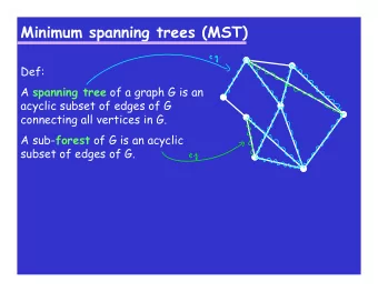
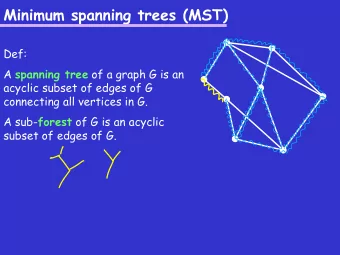
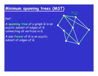
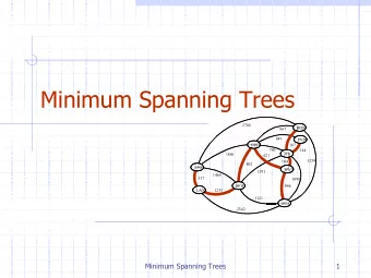
Minimum Spanning Trees A tree is a connected graph with no cycles. A spanning tree is a subgraph of G which has the same set of vertices of G and is a tree. A minimum spanning tree of a weighted graph G is the spanning tree of G whose edges sum to minimum weight. There can be more than one minimum spanning tree in a graph → consider a graph with identical weight edges.

(c) (b) (a)

Why Minimum Spanning Trees? The minimum spanning tree problem has a long history – the first algorithm dates back at least to 1926!. Minimum spanning tree is always taught in algorithm courses since (1) it arises in many applications, (2) it is an important example where greedy algorithms always give the optimal answer, and (3) Clever data structures are necessary to make it work. In greedy algorithms, we make the decision of what next to do by selecting the best local option from all available choices – without regard to the global structure.

Applications of Minimum Spanning Trees Minimum spanning trees are useful in constructing networks, by describing the way to connect a set of sites using the smallest total amount of wire. Minimum spanning trees provide a reasonable way for clustering points in space into natural groups. What are natural clusters in the friendship graph?

Minimum Spanning Trees and Net Partitioning One of the war stories in the text describes how to partition a graph into compact subgraphs by deleting large edges from the minimum spanning tree. (a) (b) (c) (d)

Minimum Spanning Trees and TSP When the cities are points in the Euclidean plane, the minimum spanning tree provides a good heuristic for traveling salesman problems. The optimum traveling salesman tour is at most twice the length of the minimum spanning tree. The Option Traveling System tour is at most twice the length of the minimum spanning tree. Note: There can be more than one minimum spanning tree considered as a group with identical weight edges.

Prim’s Algorithm If G is connected, every vertex will appear in the minimum spanning tree. If not, we can talk about a minimum spanning forest. Prim’s algorithm starts from one vertex and grows the rest of the tree an edge at a time. As a greedy algorithm, which edge should we pick? The cheapest edge with which can grow the tree by one vertex without creating a cycle.

Prim’s Algorithm (Pseudocode) During execution each vertex v is either in the tree, fringe (meaning there exists an edge from a tree vertex to v ) or unseen (meaning v is more than one edge away). Prim-MST(G) Select an arbitrary vertex s to start the tree from. While (there are still non-tree vertices) Select the edge of minimum weight between a tree Add the selected edge and vertex to the tree T prim . This creates a spanning tree, since no cycle can be introduced, but is it minimum?

Prim’s Algorithm in Action 5 7 6 2 5 1 2 4 2 4 9 3 3 3 5 7 1 5 7 4 2 6 4 12 A A A G Prim(G,A) Kruskal(G)

Why is Prim Correct? We use a proof by contradiction: Suppose Prim’s algorithm does not always give the minimum cost spanning tree on some graph. If so, there is a graph on which it fails. And if so, there must be a first edge ( x, y ) Prim adds such that the partial tree V ′ cannot be extended into a minimum spanning tree.

x y x y s s v1 v2 (b) (a) But if ( x, y ) is not in MST ( G ) , then there must be a path in MST ( G ) from x to y since the tree is connected. Let ( v, w ) be the first edge on this path with one edge in V ′ Replacing it with ( x, y ) we get a spanning tree. with smaller weight, since W ( v, w ) > W ( x, y ) . Thus you did not have the MST!!

Prim’s Algorithm is correct! Thus we cannot go wrong with the greedy strategy the way we could with the traveling salesman problem.

How Fast is Prim’s Algorithm? That depends on what data structures are used. In the simplest implementation, we can simply mark each vertex as tree and non-tree and search always from scratch: Select an arbitrary vertex to start. While (there are non-tree vertices) select minimum weight edge between tree and fringe add the selected edge and vertex to the tree This can be done in O ( nm ) time, by doing a DFS or BFS to loop through all edges, with a constant time test per edge, and a total of n iterations.

Prim’s Implementation To do it faster, we must identify fringe vertices and the minimum cost edge associated with it fast. prim(graph *g, int start) { int i; (* counter *) edgenode *p; (* temporary pointer *) bool intree[MAXV]; (* is the vertex in the tree yet? *) int distance[MAXV]; (* distance vertex is from start *) int v; (* current vertex to process *) int w; (* candidate next vertex *) int weight; (* edge weight *) int dist; (* best current distance from start *) for (i=1; i < = g − > nvertices; i++) { intree[i] = FALSE; distance[i] = MAXINT; parent[i] = -1; } distance[start] = 0;

v = start; while (intree[v] == FALSE) { intree[v] = TRUE; p = g − > edges[v]; while (p ! = NULL) { w = p − > y; weight = p − > weight; if ((distance[w] > weight) && (intree[w] == FALSE)) { distance[w] = weight; parent[w] = v; } p = p − > next; } v = 1; dist = MAXINT; for (i=1; i < = g − > nvertices; i++) if ((intree[i] == FALSE) && (dist > distance[i])) { dist = distance[i]; v = i; } } }

Prim’s Analysis Finding the minimum weight fringe-edge takes O ( n ) time – just bump through fringe list. After adding a vertex to the tree, running through its adjacency list to update the cost of adding fringe vertices (there may be a cheaper way through the new vertex) can be done in O ( n ) time. Total time is O ( n 2 ) .

Kruskal’s Algorithm Since an easy lower bound argument shows that every edge must be looked at to find the minimum spanning tree, and the number of edges m = O ( n 2 ) , Prim’s algorithm is optimal in the worst case. Is that all she wrote? The complexity of Prim’s algorithm is independent of the number of edges. Can we do better with sparse graphs? Yes! Kruskal’s algorithm is also greedy. It repeatedly adds the smallest edge to the spanning tree that does not create a cycle.

Kruskal’s Algorithm in Action 5 7 6 2 5 1 2 4 2 4 9 3 3 3 5 7 1 5 7 4 2 6 4 12 A A A G Prim(G,A) Kruskal(G)

Why is Kruskal’s algorithm correct? Again, we use proof by contradiction. Suppose Kruskal’s algorithm does not always give the minimum cost spanning tree on some graph. If so, there is a graph on which it fails. And if so, there must be a first edge ( x, y ) Kruskal adds such that the set of edges cannot be extended into a minimum spanning tree. When we added ( x, y ) there previously was no path between x and y , or it would have created a cycle Thus if we add ( x, y ) to the optimal tree it must create a cycle. At least one edge in this cycle must have been added after ( x, y ) , so it must have a heavier weight.

Deleting this heavy edge leave a better MST than the optimal tree? A contradiction!

How fast is Kruskal’s algorithm? What is the simplest implementation? • Sort the m edges in O ( m lg m ) time. • For each edge in order, test whether it creates a cycle the forest we have thus far built – if so discard, else add to forest. With a BFS/DFS, this can be done in O ( n ) time (since the tree has at most n edges). The total time is O ( mn ) , but can we do better?

Fast Component Tests Give Fast MST Kruskal’s algorithm builds up connected components. Any edge where both vertices are in the same connected compo- nent create a cycle. Thus if we can maintain which vertices are in which component fast, we do not have test for cycles! • Same component( v 1 , v 2 ) – Do vertices v 1 and v 2 lie in the same connected component of the current graph? • Merge components( C 1 , C 2 ) – Merge the given pair of connected components into one component.

Fast Kruskal Implementation Put the edges in a heap count = 0 while ( count < n − 1) do get next edge ( v, w ) if (component (v) � = component(w)) add to T component (v)=component(w) If we can test components in O (log n ) , we can find the MST in O ( m log m ) ! Question: Is O ( m log n ) better than O ( m log m ) ?