Lecture 11: Coding and Entropy. David Aldous March 9, 2016 [show - PowerPoint PPT Presentation

Lecture 11: Coding and Entropy. David Aldous March 9, 2016

[show xkcd] This lecture looks at a huge field with the misleading name Information Theory – course EE 229A. Start with discussing a concept of entropy . This word has several different-but-related meanings in different fields of the mathematical sciences; we focus on one particular meaning. Note: in this lecture coding has a special meaning – representing information in some standard digital way for storage or communication.

For a probability distribution over numbers – Binomial or Poisson, Normal or Exponential – the mean or standard distribution are examples of “statistics” – numbers that provide partial information about the distribution. Consider instead a probability distribution over an arbitrary finite set S p = ( p s , s ∈ S ) Examples we have in mind for S are Relative frequencies of letters in the English language

Relative frequencies of letters in the English language Relative frequencies of words in the English language Relative frequencies of phrases or sentences in the English language [show Google Ngram] Relative frequencies of given names [show] For such S mean does not make sense. But statistics such as � p 2 s s and � − p s log p s s do make sense.

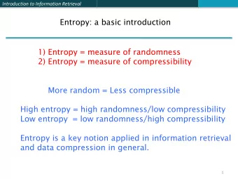
s p 2 What do these particular statistics � s and − � s p s log p s measure? [board]: spectrum from uniform distribution to deterministic. Interpret as “amount of randomness” or “amount of non-uniformity”. First statistic has no standard name. Second statistic: everyone calls it the entropy of the probability distribution p = ( p s , s ∈ S ). For either statistic, a good way to interpret the numerical value is as an “effective number” N eff – the number such that the uniform distribution on N eff categories has the same statistic. [show effective-names.pdf – next slide] For many purposes the first statistic is most natural – e.g. the chance two random babies born in 2013 are given the same name. The rest of this lecture is about contexts where the entropy statistic is relevant.

Effective Number of Names (1/sumofsquares) over time Effective Number of Names (exp(entropy)) over time female 2000 female male 500 male 1500 400 effective number of names effective number of names 300 1000 200 500 100 0 0 1880 1900 1920 1940 1960 1980 2000 1880 1900 1920 1940 1960 1980 2000 year year Frequency*Effective # of 'common' female names over time Frequency*Effective # of male names over time 8 Tatiana (2009) 30 William (2009) Peyton (1999) Andrew (1999) Justin (1989) Brenda (1989) frequency of name * eff.# of names this year frequency of name * eff.# of names this year Michael (1979) Candice (1979) 25 David (1969) Annette (1969) John (1959) Ruth (1959) 6 20 4 15 10 2 5 0 0 1880 1900 1920 1940 1960 1980 2000 1880 1900 1920 1940 1960 1980 2000 year year

In our context it is natural to take logs to base 2. So if we pick a word uniform at random from the 2000 most common English words, this random process has entropy log 2 2000 ≈ 11, and we say this as “11 bits of entropy”. [show xkcd again] Of course we can’t actually pick uniformly “out of our head” but the notion of “effective population size” holds.

You may have seen the second law of thermodynamics [show] The prominence of entropy in this “physical systems” context has led to widespread use and misuse of the concept in other fields. This lecture is about a context where it is genuinely a central concept.

A simple coding scheme is ASCII [show] In choosing how to code a particular type of data there are three main issues to consider. May want coded data to be short, for cheaper storage or communication: data compression May want secrecy: encryption May want to be robust under errors in data transmission: error-correcting code [comment on board] At first sight these are quite different issues, but . . . . . .

Here is a non-obvious conceptual point. Finding good codes for encryption is (in principle) the same as finding good codes for compression. Here “the same as” means “if you can do one then you can do the other”. In this and the next 3 slides I first give a verbal argument for this assertion, and this argument motivates subsequent mathematics. A code or cipher transforms plaintext into ciphertext . The simplest substitution cipher transforms each letter into another letter. Such codes – often featured as puzzles in magazines – are easy to break using the fact that different letters and letter-pairs occur in English (and other natural languages) with different frequencies. A more abstract viewpoint is that there are 26! possible “codebooks” but that, given a moderately long ciphertext, only one codebook corresponds to a meaningful plaintext message.

Now imagine a hypothetical language in which every string of letters like QHSKUUC . . . had a meaning. In such a language, a substitution cipher would be unbreakable, because an adversary seeing the ciphertext would know only that it came from of 26! possible plaintexts, and if all these are meaningful then there would be no way to pick out the true plaintext. Even though the context of secrecy would give hints about the general nature of a message – say it has military significance, and only one in a million messages has military significance – that still leaves 10 − 6 × 26! possible plaintexts.

Returning to English language plaintext, let us think about what makes a compression code good. It is intuitively clear that for an ideal coding we want each possible sequence of ciphertext to arise from some meaningful plaintext (otherwise we are wasting an opportunity); and it is also intuitively plausible that we want the possible ciphertexts to be approximately equally likely (this is the key issue that the mathematics deals with).

Suppose there are 2 1000 possible messages, and we’re equally likely to want to communicate each of them. Suppose we have a public ideal code for compression , which encodes each message as a different 1000-bit string, Now consider a substitution code based on the 32 word “alphabet” of 5-bit strings. Then we could encrypt a message by (i) apply the public algorithm to get a 1000-bit string; (ii) then use the substitution code, separately on each 5-bit block. An adversary would know we had used one of the 32! possible codebooks and hence know that the message was one of a certain set of 32! plaintext messages. But, by the “approximately equally likely” part of the ideal coding scheme, these would be approximately equally likely, and again the adversary has no practical way to pick out the true plaintext. Conclusion: given a good public code for compression, one can easily convert it to a good code for encryption.

Math theory The basis of the mathematical theory is that we model the source of plaintext as random “characters” X 1 , X 2 , X 3 , . . . in some “alphabet”. It is important to note that we do not model them as independent (even though I use independence as the simplest case for mathematical calculation later) since real English plaintext obviously lacks independence. Instead we model the sequence ( X i ) as a stationary process , which basically means that there is some probability that three consecutive characters are CHE, but this probability does not depend on position in the sequence, and we don’t make any assumptions about what the probability is.

For any sequence of characters ( x 1 , . . . , x n ) there is a likelihood ℓ ( x 1 , . . . , x n ) = P ( X 1 = x 1 , . . . , X n = x n ) . The stationarity assumption is that for each “time” t (really this is “position in the sequence”) P ( X t +1 = x 1 , . . . , X t + n = x n ) = P ( X 1 = x 1 , . . . , X n = x n ) . (1) Consider the empirical likelihood L n = ℓ ( X 1 , . . . , X n ) which is the prior chance of seeing the sequence that actually turned up. The central result (Shannon-McMillan-Breiman theorem: STAT205B) is

The asymptotic equipartition property (AEP) . For a stationary ergodic source, there is a number E nt , called the entropy rate of the source, such that for large n , with high probability − log L n ≈ n × E nt . It is conventional to use base 2 logarithms in this context, to fit nicely with the idea of coding into bits. I will illustrate by simple calculations in the IID case, but it’s important that the AEP is true very generally. We will see the connection with coding later.

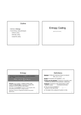
For n tosses of a hypothetical biased coin with P ( H ) = 2 / 3 , P ( T ) = 1 / 3, the most likely sequence is HHHHHH . . . HHH , which has likelihood (2 / 3) n , but a typical sequence will have about 2 n / 3 H’s and about n / 3 T’s, and such a sequence has likelihood ≈ (2 / 3) 2 n / 3 (1 / 3) n / 3 . So log 2 L n ≈ n ( 2 2 3 + 1 1 3 log 2 3 log 2 3 ) . Note in particular that log-likelihood behaves differently from the behavior of sums, where the CLT implies that a “typical value” of a sum is close to the most likely individual value. Recall that the entropy of a probability distribution q = ( q j ) is defined as the number � E ( q ) = − q j log 2 q j . (2) j