Learning the dynamics of biological networks Thierry Mora - PowerPoint PPT Presentation
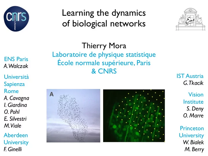
Learning the dynamics of biological networks Thierry Mora Laboratoire de physique statistique ENS Paris cole normale suprieure, Paris A. Walczak & CNRS IST Austria Universit G. Tkacik Sapienza Rome Vision A. Cavagna
⇨ dynamical maximum entropy maximum entropy gives a “steady-state” picture. what about the dynamics? ad hoc dynamics such as Glauber, Metropolis may be wrong P ( σ 1 , . . . , σ T ) (a) solution: maximum entropy over trajectories t t+1 t+2 i σ t 0 constraints on cross-time correlations, e.g. h σ t j i − A “action” ⇢ 0 1 P ( σ 1 , . . . , σ T ) = 1 J t − t 0 @ X i σ t 0 σ t Z exp A j ij i,j,t,t 0 not the same as: 2 3 1 J t − t 0 X P ( σ i,t |{ σ j,t 0 } t 0 <t ) = Z ( { σ j,t 0 } t 0 <t ) exp 4 h i σ i,t + σ i,t σ j,t 0 5 ij j,t 0 <t
example 1: flocks of birds
example 1: flocks of birds
aligned collective motion ξ fluctuations around main orientation strong polarization r φ = 1 v ∑ r domains i ~ 0.95 N v i i
a maximum entropy model for birds velocity of bird v i , s i = � v i / k � v i k � �
a maximum entropy model for birds velocity of bird v i , s i = � v i / k � v i k � � constrain correlation functions C ij = h � s j i s i � 0 1 s N ) = 1 A = 1 @X P ( � Z exp Z exp( − H ) s 1 , . . . , � J ij � s i � s j ij (Heisenberg model on lattice)
a maximum entropy model for birds velocity of bird v i , s i = � v i / k � v i k � � constrain correlation functions C ij = h � s j i s i � 0 1 s N ) = 1 A = 1 @X P ( � Z exp Z exp( − H ) s 1 , . . . , � J ij � s i � s j ij (Heisenberg model on lattice)
a maximum entropy model for birds velocity of bird v i , s i = � v i / k � v i k � � constrain correlation functions C ij = h � s j i s i � 0 1 s N ) = 1 A = 1 @X P ( � Z exp Z exp( − H ) s 1 , . . . , � J ij � s i � s j ij (Heisenberg model on lattice) derives from Langevin eqn, equilavent to “social” model, similar to Vicsek’s N d ⇤ dt = − ⇥ H s i X + ⇤ � i ( t ) = s j + ⇤ � i ( t ) J ij ⇤ ⇥⇤ s i noise j=1 alignment (does not mean that’s the only possible dynamics, or the true one)
parametrization ⇢ J if j is one i’s n c first neighbors then symmetrized J ij = otherwise 0
parametrization ⇢ J if j is one i’s n c first neighbors then symmetrized J ij = otherwise 0 N Equivalent to maximum C int = 1 1 X X h � s j i s i � entropy with constraint on N n c i =1 j ∈ V ( i ) single snapshot — spatial averaging instead of ensemble averaging
predicting correlation functions interaction range correlation range perpendicular correlation long-range order from local interactions
predicting correlation functions 4-bird correlation function interaction range B Correlation C 4 (r 1 ,r 2 ) i k Data r 2 Model 0.004 r 1 r 1 l j correlation 0.002 range perpendicular correlation r 1 =0.5 0 0 10 20 30 40 Distance r 2 (m) long-range order from local interactions
interaction range metric or topological ?
interaction range r c r 1 metric or topological ?
interaction range r c r 1 metric or topological ? r c r 1
interaction range r c n c = 6 r 1 metric or topological ? r c r 1
interaction range r c n c = 6 r 1 metric or topological ? r c n c = 6 r 1
interaction range r c n c = 6 r 1 metric or topological ? r c n c = 6 r 1 n c -1/3 r 1
interaction range r c n c = 6 r 1 metric or topological ? r c n c = 6 r 1 n c ~ (r c / r 1 ) 3 n c -1/3 n c r 1 r 1
answer: interaction is topological not metric E 1 -1/3 Interaction range n c 0.5 0 0.6 0.8 1 1.2 1.4 1.6 1.8 sparseness r 1 (m) Bialek et al PNAS 2012
answer: interaction is topological not metric n c ~ 21 does not depend on flock density flock size E D 1 60 -1/3 Interaction range n c Interaction range n c 40 0.5 20 0 0 0 20 40 60 80 0.6 0.8 1 1.2 1.4 1.6 1.8 Flock size (m) sparseness r 1 (m) Bialek et al PNAS 2012
dynamics (may) matter we’ve assumed that neighborhoods are fixed but birds may exchange neighbors fast
dynamics (may) matter we’ve assumed that neighborhoods are fixed but birds may exchange neighbors fast
dynamics (may) matter we’ve assumed that neighborhoods are fixed but birds may exchange neighbors fast the effective number of interaction partners could be larger than the instantaneous one.
dynamics (on bird orientations) constrain and h s t i s t h s t i s t +1 j i i j P ( s 1 , . . . , s T ) = 1 exp ( − A ) ˆ Z A = − 1 ⇣ ⌘ J (1) j + J (2) X X ij ; t s t +1 ij ; t s t i s t s t “action” i j 2 t i 6 = j
dynamics (on bird orientations) constrain and h s t i s t h s t i s t +1 j i i j P ( s 1 , . . . , s T ) = 1 exp ( − A ) ˆ Z A = − 1 ⇣ ⌘ J (1) j + J (2) X X ij ; t s t +1 ij ; t s t i s t s t “action” i j 2 t i 6 = j in spin-wave approximation, equivalent to “collective random walk” � � n s A and M functions of J (1) and J (2) ~ ⇡
dynamics (on bird orientations) constrain and h s t i s t h s t i s t +1 j i i j P ( s 1 , . . . , s T ) = 1 exp ( − A ) ˆ Z A = − 1 ⇣ ⌘ J (1) j + J (2) X X ij ; t s t +1 ij ; t s t i s t s t “action” i j 2 t i 6 = j in spin-wave approximation, equivalent to “collective random walk” alignment strength � � n s temperature ~ ⇡ Langevin equation
inferring out-of-equilibrium behavior infering J, n c , and a third parameter, the “temperature” T and similar eq. for T C int − C s + G s − G int J n c = 1 δ t 2 C int − C 0 int − C s
inferring out-of-equilibrium behavior infering J, n c , and a third parameter, the “temperature” T and similar eq. for T C int − C s + G s − G int J n c = 1 δ t 2 C int − C 0 int − C s if equilibrium – slowly evolving and symmetric n ij – then one recovers the same result as the Heisenberg model, with J ← J / T 0 1 s N ) = 1 @ J X P ( � Z exp s 1 , . . . , � n ij � s i � s j A T ij
test on simulated data simulation of 2D topological model with Voronoi neighbors µ is a parameter quantifying how fast birds change neighbors 20 dynamical inference 3.8 static inference 15 static inference n ∗ 3.6 c overestimates 0 10 20 number of partners n ∗ 10 c true value 5 dynamic static 0 0 0.2 0.4 0.6 0.8 1 µ at large µ, Cavagna et al PRE 2014 dynamical maximum entropy works, static maximum entropy doesn’t
the retina multielectrode array recordings
the stimulus
the stimulus
binary neurons raster → binary variables N ~ 150 neurons σ i = 0 , 1 10 ms Marre et al. J. Neurosci. 2012
neuron activities are correlated Schneidman et al, Nature 2005 independenc P 1 ( σ ) = 1 P i h i σ i Z e total number of spikes Ising model P 2 ( σ ) = 1 P i h i σ i + P ij J ij σ i σ j Z e
neuron activities are correlated Schneidman et al, Nature 2005 independenc P 1 ( σ ) = 1 P i h i σ i Z e total number of spikes Ising model P 2 ( σ ) = 1 P i h i σ i + P ij J ij σ i σ j Z e goal: build the thermodynamics of this correlated system from data
building the density of states evaluate by modelling or by frequency counting P ( σ 1 , . . . , σ N )
building the density of states evaluate by modelling or by frequency counting P ( σ 1 , . . . , σ N ) define “energy” through Boltzmann law P = 1 E = − log P Z e − E/k B T
building the density of states evaluate by modelling or by frequency counting P ( σ 1 , . . . , σ N ) define “energy” through Boltzmann law P = 1 E = − log P Z e − E/k B T now consider the distribution of energies E C ( E ) = number of states with E ( σ ) < E
building the density of states evaluate by modelling or by frequency counting P ( σ 1 , . . . , σ N ) define “energy” through Boltzmann law P = 1 E = − log P Z e − E/k B T now consider the distribution of energies E C ( E ) = number of states with E ( σ ) < E define a microcanonical entropy : S ( E ) = log C ( E ) Mora Bialek J. Stat. Phys. 2011
density of states just counting states Maximum entropy model (under natural movie stimulus) Tkacik Mora Marre Amodei Berry Bialek, arxiv 2014
Zipf’s law (interlude) Zipf 1949
Zipf’s law (interlude) Probability P ( E in log scale) ~ cumulative distribution Zipf 1949
what does S(E) = E mean?
what does S(E) = E mean? what’s the probability of a given energy? how many states at E probability of a state at E P ( E ) ≈ e S − E constant!
what does S(E) = E mean? what’s the probability of a given energy? how many states at E probability of a state at E (note: only works P ( E ) ≈ e S − E constant! if exponent is = 1 )
what does S(E) = E mean? what’s the probability of a given energy? how many states at E probability of a state at E (note: only works P ( E ) ≈ e S − E constant! if exponent is = 1 ) in usual thermodynamics… E scales with N its fluctuations scale with N heat capacity C = Var( E ) ∼ N C / N diverges at 2nd order transition critical point ( e.g. 2D Ising model)
what does S(E) = E mean? what’s the probability of a given energy? how many states at E probability of a state at E (note: only works P ( E ) ≈ e S − E constant! if exponent is = 1 ) in usual thermodynamics… E scales with N its fluctuations scale with N heat capacity C = Var( E ) ∼ N C / N diverges at 2nd order transition critical point ( e.g. 2D Ising model) link to information theory “surprise” (Shannon 1948) E = − log P equipartition theorem (valid for independent units): almost all codewords we see have the same surprise ~ entropy basis for compression
specific heat let’s add a spurious temperature — one direction in parameter space 1 Z ( T ) e − E/T P T ( σ ) = C = Var T ( E/T ) = Var T ( − log P ) ( T = 1 corresponds to the real ensemble)
specific heat let’s add a spurious temperature — one direction in parameter space 1 Z ( T ) e − E/T P T ( σ ) = C = Var T ( E/T ) = Var T ( − log P ) ( T = 1 corresponds to the real ensemble)
specific heat let’s add a spurious temperature — one direction in parameter space 1 Z ( T ) e − E/T P T ( σ ) = C = Var T ( E/T ) = Var T ( − log P ) ( T = 1 corresponds to the real ensemble) Neural network Tkacik Mora Marre Amodei Berry Bialek, arxiv 2014
dynamical criticality
dynamical approach 10 ms σ t
dynamical approach 10 ms σ t P ( σ 1 , . . . , σ L ) proposal: consider statistics over trajectories t t+1 t+2
dynamical approach 10 ms σ t P ( σ 1 , . . . , σ L ) proposal: consider statistics over trajectories t t+1 t+2 1 calculate specific heat c = define NL Var( E ) E = − log P ( { σ i,t } )
link to dynamical criticality: branching process N p ij Y Y p i ( t ) σ i,t [1 − p i ( t )] 1 − σ i,t P ( { σ i,t } ) = t i =1 Y p i ( t ) = 1 − (1 − p ij ) σ i,t − 1 Beggs & Plenz 2003 t j branching parameter: ω = 1 X p ij N ij
link to dynamical criticality: branching process N p ij Y Y p i ( t ) σ i,t [1 − p i ( t )] 1 − σ i,t P ( { σ i,t } ) = t i =1 Y p i ( t ) = 1 − (1 − p ij ) σ i,t − 1 Beggs & Plenz 2003 t j branching parameter: ω = 1 X p ij N ij Shew Yang Petermann Roy Plenz 2009
model for multi-neuron spike trains sampling 2 N states is hard enough; here 2 NL states — we need models let’s do something simple X total number of spikes K t = σ i,t i is informative of collective behaviour Tkacik Marre Mora Amodei Berry Bialek, JSTAT 2013 independent neutrons
model for multi-neuron spike trains sampling 2 N states is hard enough; here 2 NL states — we need models let’s do something simple X total number of spikes K t = σ i,t i is informative of collective behaviour Tkacik Marre Mora Amodei Berry Bialek, JSTAT 2013 maximum entropy model with constrains on temporal correlations of K | t − t 0 | < v P ( K t , K t 0 ) independent ⬄ all neurons behave the same neutrons
model for multi-neuron spike trains sampling 2 N states is hard enough; here 2 NL states — we need models let’s do something simple X total number of spikes K t = σ i,t i is informative of collective behaviour Tkacik Marre Mora Amodei Berry Bialek, JSTAT 2013 maximum entropy model with constrains on temporal correlations of K | t − t 0 | < v P ( K t , K t 0 ) independent ⬄ all neurons behave the same neutrons “Energy” v X X X E = − h ( K t ) − J u ( K t , K t + u ) t t u =1
solving the problem v X X X E = − h ( K t ) − J u ( K t , K t + u ) t t u =1 define a “super-variable” X t = ( K t , K t +1 , . . . , K t + v − 1 ) now becomes a 1D model "X # P ( { X t } ) = 1 X Z exp H ( X t ) + W ( X t , X t +1 ) t t can be solved by transfer matrices ( aka forward backward algorithm, or belief propagation in 1D)
model predicts avalanche dynamics − 1 b. 10 − 2 10 Probability − 3 10 observed v = 0 v = 1 − 4 v = 2 10 v = 3 v = 4 v = 5 − 5 10 0 1 2 3 10 10 10 10 Avalanche size (number of spikes)
model predicts avalanche dynamics − 1 b. 10 − 2 10 Probability − 3 10 observed v = 0 v = 1 − 4 v = 2 10 v = 3 v = 4 v = 5 − 5 10 0 1 2 3 10 10 10 10 Avalanche size (number of spikes) NB: no power laws in avalanche statistics
thermodynamics of spike trains i E = − log P ( { σ i,t } ) N 1 Z ( T ) e − E/T P T ( σ ) = t L C = Var T ( E/T ) a. b. v = 0 N = 5 20 20 v = 1 N = 10 v = 2 N = 20 v = 3 N = 30 C(T)/NL 15 v = 4 15 C(T)/NL N = 40 N = 50 c ( β ) N = 61 10 10 N = 97 N = 185 5 5 0 0 0.9 1 1.1 0.9 0.95 1 1.05 1.1 Temperature 1 / β 1 / β T T v = temporal range Mora Deny Marre PRL 2015
thermodynamics of spike trains i (salamander) E = − log P ( { σ i,t } ) N static 1 Z ( T ) e − E/T P T ( σ ) = ! t L C = Var T ( E/T ) a. b. v = 0 N = 5 20 20 v = 1 N = 10 v = 2 N = 20 v = 3 dynamic N = 30 C(T)/NL 15 v = 4 15 C(T)/NL N = 40 (rat) N = 50 c ( β ) N = 61 10 10 N = 97 N = 185 5 5 0 0 0.9 1 1.1 0.9 0.95 1 1.05 1.1 Temperature 1 / β 1 / β T T v = temporal range Mora Deny Marre PRL 2015
scaling with network size b. Var(surprise) /NL 20 v = 0 v = 1 v = 2 v = 3 15 v = 4 v = 5 10 5 0 0 100 200 Network size N 1.2 v = 0 Peak temperature 1 / β c v = 1 NL v = 2 v = 3 1.15 v = 4 v = 5 1.1 1.05 T 1 0 50 100 150 200 Network size N
conclusions stationary maximum entropy models may capture emergent behaviour in biological data but dynamic framework may be necessary to get parameters right in neural systems, heat capacity = useful indicator of critical properties critical signature enhanced by dynamical approach application to other biological contexts?
random flickering checkerboard
Recommend
More recommend
Explore More Topics
Stay informed with curated content and fresh updates.
