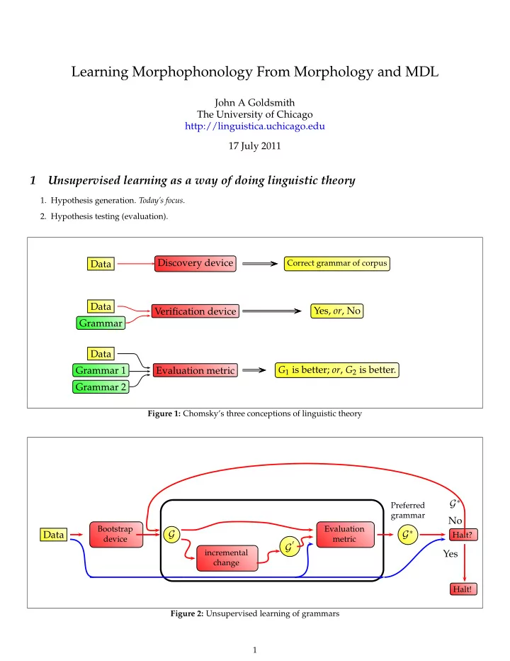

Learning Morphophonology From Morphology and MDL John A Goldsmith The University of Chicago http://linguistica.uchicago.edu 17 July 2011 1 Unsupervised learning as a way of doing linguistic theory 1. Hypothesis generation. Today’s focus . 2. Hypothesis testing (evaluation). Discovery device Data Correct grammar of corpus Data Yes, or , No Verification device Grammar Data G 1 is better; or , G 2 is better. Grammar 1 Evaluation metric Grammar 2 Figure 1: Chomsky’s three conceptions of linguistic theory G ∗ Preferred grammar No Bootstrap Evaluation G ∗ G Data Halt? device metric ′ G incremental Yes change Halt! Figure 2: Unsupervised learning of grammars 1
2 Unsupervised learning of morphology: the Linguistica project (2001) 2.1 Working on the unsupervised learning of natural language morphology. Why? What is the task, then? Take in a raw corpus, and produce a morphology. What is a morphology? The answer to that depends on what linguistic problems we want to solve. Let’s start with the simplest: analysis of words into morphs (and eventually into morphemes). Solution looks like an FSA, then. Examples: English, French, Swahili. An FSA is a set of vertices (or nodes), a set of edges, and for each edge a label and a probability, where the sum of the probabilities of the edges leaving each node sums to 1.0. 1. English morphology: morphemes on edges of a finite-state automaton ly proud, loud l a c i / s s e l / l u lord, hard, friend f ship s buddh, special, capital ist ∅ ment, er, ion, ing, al dog, boy, girl cultiv, calcul ate ∅ ed jump, walk, love, move s ing Figure 3: English morphology: morphemes on edges Pose the problem as an optimization problem: quantitative data that can be measured, but provides qualitatively special points in a continuous world of measurement. Turning this into a linguistic project Some details on the MDL model; no time to talk about the search methods. We can use the term length (of something) to mean the number of bits = amount of information needed to specify it. Except where indicated, the probability distribution(s) involved are from maximum likelihood models. The length of an FSA is the number of bits needed to specify it, and it equals the sum of these things: 1. List of morphemes: assigning the phonological cost of establishing a lean class of morphemes. Avoid redundancy; minimize multiple use identical strings. The probability distribution here is over phonemes (letters). | t | + 1 ∑ ∑ − log pr phono ( t i | t i − 1 ) t ∈ morphemes i = 1 2. List of nodes v : the cost of morpheme classes ∑ − log pr ( v ) v ∈ Vertices 2
s nouns: chien, lit, homme, femme ∅ ment dirige , sav , suiv adverbs ant e s rond , espagnol , grand ∅ ∅ ale amic, norm, g´ en´ er- ales al aux a aient d ´ evelopp , regroup , exerc ait ant and many more Figure 4: French 3. List of edges e : the cost of morphological structure: avoid morphological analysis except where it is helpful. ∑ − log pr ( v 1 ) − log pr ( v 2 ) − log pr ( m ) e ( v 1 , v 2 , m ) ∈ Edges (I leave off the specification of the probabilities on the FSA itself, which is also a cost that is specified in bits.) In addition, a word generated by the morphology is the same as a path through the FSA. Pr ( w ) = product of the choice probabilities of for w ’s path. So: for a given corpus, Linguistica seeks the FSA for which the description length of the corpus given the FSA is minimized, which is something that can be done in an entirely language-independent and unsupervised fashion. ∅ walk s A B C ed jump ing 3
b Interpreting this graph : The x-axis and y-axis both quantities bits | g | − logpr ( d | g ( x )) measured in bits . The x-axis marks how many bits we are allowed to use to write a grammar to describe the data: the more bits we are allowed, the better our description will be, until the point where we are over-fitting the data. Thus each minimum point along the x-axis represents a possible grammar-length; but for any given length l , we care only about the grammar g that assigns the highest probability to the data, i.e., the best grammar. The red line indicates how many bits of data are | g ( x ) | = length of g(x) left unexplained by the grammar, a quantity which is equal to -1 * log probability of the data as assigned by the grammar. − logpr ( d | g ( x )) The blue line shows the sum of these two qunantities (which is the conditional description length of the data). The black line x Capacity (bits) gives the length of the grammar. Figure 5: MDL optimization 3cTop part of Linguistica ’s output from 600,000 words of English: Signature exemplar count Stem count ∅ − s pagoda 20,615 1330 ‘ s − ∅ Cambodia 30,100 683 ∅ − ly zealous 14,441 479 ∅ − ed − ing − s yield 6,235 123 ‘ s − ∅ − s youngster 4,572 121 e − ed − es − ing zon 3,683 72 ies − y weekl 2,279 124 ∅ − ly − ness wonderful 2,883 64 ∅ − es birch 2,472 96 ∅ − ed − er − ing − s pretend 957 19 ence − ent virul 571 37 ∅ − ed − es − ing witness 638 18 . . . 3 Learning (morpho)phonology from morphology It never ceases to amaze me how hard it is to develop an explicit algorithm to perform a simple linguistic task, even one that is purely formal. Surely succeeding in that task is a major goal of linguistics. Morphology treats the items in the lexicon of a language (finite or infinite; let’s assume finite to make the math easier). Any given analysis divides the lexicon up into a certain number of subgroups. If there are n subgroups, each equally likely, in a lexicon of size V ( V for vocabulary ), then marking each word costs − log 2 n V . (If the groups are not equally likely, and the i th group has n i members, then marking a word as being in that group costs − log 2 n i n i . Each word in the i th group V = log 2 V needs to be marked, and all of those markings together costs n i × log 2 V n i . If we can collapse two subgroups analytically, then we savea lot of bits. How many? If the two groups are equal-sized, then we save 1 bit for each item. Why? Suppose we have two groups, g 1 and g 2 of 100 words out of a vocabulary of 1000 words. Each item in those two groups is marked in the lexicon at a cost of log 2 1000 100 ≈ 3.3 bits ; 200 such words costs us 200 × 3.32 bits = 664 bits. If they were all treated as part of a single category, the cost of pointing to the larger category would be − log 2 200 1000 = 2.32 bits , so we would pay a total of 200 × 2.32 = 464 bits . for a total saving of 200 bits. We actually compute how complex an analysis is. And the morphological analysis that Linguistica provides can be made “cheaper” by decreasing the number of distinct patterns it contains, by adding a (morpho)phonology component after the morphology. But how can we discover it automatically? 4
3.1 English verb Regular verbal patterns e -final verbal pattern jump walk move love hate jumped walked (1) (2) moved loved hated jumping walking moving loving loved jumps walks moves loves loves s -final pattern C-doubling pattern y-final pattern push miss veto tap slit nag try cry lie* (3) (4) (5) pushed missed vetoed tapped slitted nagged tried cried lied pushing missing vetoing tapping slitting nagging trying crying lying pushes misses vetoes taps slits nags tries cries lies Figure 6: Some related paradigms Definition (tight) : Given an alphabet A . Define a cancella- string S string T ∆ R ( S , T ) tion operation and an inverse alphabet A − 1 : For each a ∈ A there is an element a − 1 in A − 1 such that aa − 1 = a − 1 a = e . ed jumped jumping Define an augmented alphabet A ≡ A ∩ A − 1 . A ∗ is the set ing ∅ jump jumping ing of all strings drawn from A . If we add the cancellation op- walk walk jump eration to A ∗ , then we get a free group G in which (e.g.) jump ab − 1 cc − 1 b = a . We normally denote the elements in G by walked walked jumped jumped the shortest strings in A ∗ that correspond to them. Definition (loose) : Given two strings S and T ∆ R ( S , T ) ≡ T − 1 S . whose longest common initial string is m ; ∆ L ( S , T ) ≡ ST − 1 . S = m + s 1 ; T = m + t 1 . ∆ R ( jumped , jumping ) ≡ ( jumping ) − 1 jumped = E.g. Then ( ing ) − 1 ( jump ) − 1 ( jump )( ed ) = ( ing ) − 1 ( ed ) = ∆ R ( string 1 , string 2 ) = s 1 ed t 1 ing Still, these matrix are quite similar to one another. We can formalize that observation, if we take advantage of the notion of string difference we defined just above. We extend the definition of ∆ L to Σ ∗ × Σ ∗ in this way: d ) = ∆ L ( a , c ) ∆ L ( a b , c (6) ∆ L ( b , d ) If we define ∆ L on a matrix as the item-wise application of that operation on the individual members, then we can express the difference between 6 and 7 in this way (where we indicate ∅ ∅ with a blank). See Figures 7,8 on next two pages. 3.2 Hungarian See Figure 10 below. 3.3 Spanish See Figure 9 below. 4 Conclusion Let P be a sequence of words (think P[aradigm] ) of length n . We define the quotient P ÷ Q of two sequences P , Q of the same length n as a 2 × 2 matrix, where P ÷ Q ( i , j ) ≡ ∆ L ( p i , q j ) 5
Recommend
More recommend