Learning from examples as an inverse problem E. De Vito - PowerPoint PPT Presentation
Learning from examples as an inverse problem E. De Vito Dipartimento di Matematica, Universit` a di Modena e Reggio Emilia Genova, October 30 2004 1 Plan of the talk 1. Motivations 2. Statistical learning theory and regularized least-squares
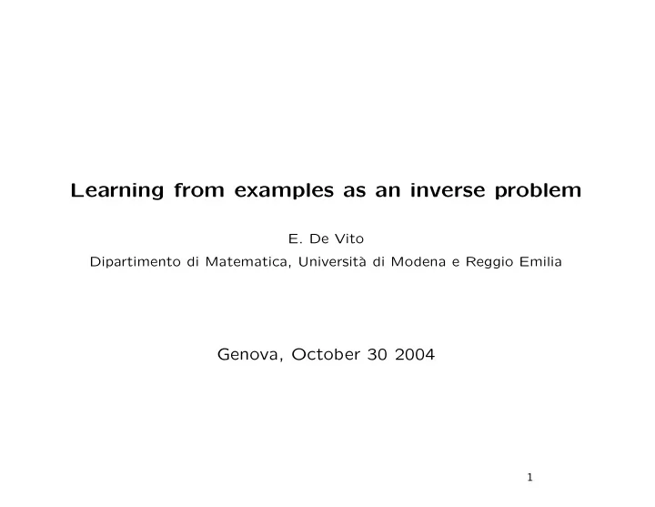
Learning from examples as an inverse problem E. De Vito Dipartimento di Matematica, Universit` a di Modena e Reggio Emilia Genova, October 30 2004 1
Plan of the talk 1. Motivations 2. Statistical learning theory and regularized least-squares algorithm 3. Linear inverse problem 4. Formal connection between 2. and 3. 5. Conclusions 2
Motivations 1. The learning theory is mainly developed in a probabilis- tic framework 2. The learning problem can be seen as the regression problem of approximating a function from sparse data and, hence, is an ill-posed problem 3. The learning algorithms are a particular instance of the regularization theory developed for ill-posed prob- lems 4. The stability of the solution is with respect to pertur- bations of the data, which play the role of noise 3
A question and a few references ———————————————————————– Is the learning theory a linear inverse problem ? ———————————————————————– 1. T.Poggio, F. Girosi, 247 Science (1990) 978-982 2. Girosi, M. Jones, T. Poggio, 7 Neural Comp. (1995) 219-269 3. V. Vapnik, Statistical learning theory , 1998 4. T. Evgeniou, M. Pontil, T. Poggio, 13 Adv.Comp.Math. (2000) 1-50 5. F. Cucker, S. Smale, Bull. Amer. Math. Soc., 39 (2002) 1-49 4
Statistical learning theory: building blocks 1. An relation between two sets of variables, X and Y . The relation is unknown , up to a set of ℓ -examples z = (( x 1 , y 1 ) , . . . , ( x ℓ , y ℓ )), and the aim of the learning theory is to describe it by means of a function f : X → Y 2. A quantitative measure of how well a function f describes the relation between x ∈ X and y ∈ Y 3. A hypothesis space H of functions encoding some a-priori knowl- edge on the relation 4. An algorithm that provides an estimator f z ∈ H for any training set z 5. A quantitative measure of the performance of the algorithm 5
1. The distribution ρ 1. The input space X is a subset of R m 2. The output space Y is R (regression) 3. The relation between x and y is described by an un- known probability distribution ρ on X × Y 6
2. The expected risk 1. The expected risk of a function f : X → Y is � X × Y ( f ( x ) − y ) 2 dρ ( x, y ) I [ f ] = and measures how well f describes the relation be- tween x and y modeled by ρ 2. The regression function � g ( x ) = Y ydρ ( y | x ) is the minimizer of the expected risk over the set of all functions f : X → R ( ρ ( y | x ) is the conditional distribution of y given x ) 7
3. The hypothesis space H The space H is a reproducing kernel Hilbert space 1. The elements of H are functions f : X → R 2. The following reproducing property holds f ( x ) = � f, K x � H K x ∈ H 3. The function f H = argmin { I [ f ] } f ∈H is the best estimator in H 8
4. The regularized least-squares algorithm 1. The examples ( x 1 , y 1 ) , . . . , ( x ℓ , y ℓ ) are drawn indepen- dently and are identically distributed according to ρ 2. Given λ > 0, the regularized least-squares estimator is ℓ { 1 f z λ = argmin ( f ( x i ) − y i ) 2 + λ � f � 2 � H } ℓ f ∈H i =1 for each training set z ∈ ( X × Y ) ℓ 3. f z λ is a random variable defined on the probability space ( X × Y ) ℓ and taking values in the Hilbert space H 9
5. Probabilistic bounds and consistency 1. A probabilistic bound B ( λ, ℓ, η ) is a function depending on the regularization parameter λ , the number ℓ of examples and the confidence level 1 − η such that � � 0 ≤ I [ f z λ ] − I [ f H ] ≤ B ( λ, ℓ, η ) Prob ≥ 1 − η z ∈ ( X × Y ) ℓ 2. B ( λ, ℓ, η ) measures the performance of the algorithm 3. B decreases as function of η and of ℓ 4. The algorithm is consistent if it is possible to choose λ , as a function of ℓ , so that, for all ǫ > 0, � � I [ f z λ ℓ ] − I [ f H ] ≥ ǫ lim Prob = 0 ℓ → + ∞ z ∈ ( X × Y ) ℓ 10
Plan of the talk 1. Motivations 2. Statistical learning and regularized least-squares algo- rithm 3. Linear inverse problem 4. Formal connection between 2. and 3. 5. Conclusions 11
The linear inverse problem 1. The operator A : H → K 2. The exact datum g ∈ K 3. The exact problem: f ∈ H such that Af = g 4. The noisy datum g δ ∈ K 5. The measure of the noise � g − g δ � K ≤ δ 6. The regularized solution of the noisy problem is { � Af − g δ � 2 K + λ � f � 2 f λ δ = argmin H } λ > 0 f ∈H 12
Comments 1. The regularization parameter λ > 0 ensures existence and uniqueness of the minimizer f λ δ 2. The theory can be extended to the case of a noisy operator A δ : H → K 3. The measures of the noise are � g − g δ � H ≤ δ 1 � A − A δ � L ( H , K ) ≤ δ 2 4. Both g and g δ belong to the same space 5. Both A and A δ belong to the same space 13
The reconstruction error � δ − f † � � f λ 1. The reconstruction error � H measures the dis- � � tance between f λ δ and the generalized solution f † = argmin { � Af − g � 2 K } f ∈H (if the minimizer is not unique, f † is the minimizer of minimal norm) 2. The parameter λ is chosen, as a function of δ , so that � � � f λ δ − f † � � lim = 0 � � δ δ → 0 � H 14
The residual 1. The residual of f λ δ is � δ − Af † � � � � Af λ � Af λ � K = δ − Pg � � � � � K where P is the projection onto the closure of Im A . 2. The residual is a weaker measure than the recon- struction error � Af − Pg � L 2 ( X,ν ) ≤ � A � L ( H , K ) � f − f H � H 15
Plan of the talk 1. Motivations 2. Statistical learning and regularized least-squares algo- rithm 3. Linear inverse problem 4. Formal connection between 2. and 3. [E. De Vito, A. Caponnetto, L. Rosasco, preprint (’04)] 5. Conclusions 16
I am looking for ... 1. An operator A : H → K 2. An exact datum g such that f H is the generalized so- lution of the inverse problem Af = g 3. A noisy datum g δ and, possibly, a noisy operator A δ 4. A noise measure δ in terms of the number ℓ of examples in the training set with the property that the algorithm is consistent, if δ converges to zero 17
The power of the square The expected risk of a function f : X → R is � X × Y ( f ( x ) − y ) 2 dρ ( x, y ) I [ f ] = � f − g � 2 = L 2 ( X,ν ) + I [ g ] where ν is the marginal distribution on X , � X f ( x ) 2 dν ( x ) � f � 2 L 2 ( X,ν ) = and g is the regression function 18
The exact problem The equation I [ f ] = � f − g � 2 L 2 ( X,ν ) + I [ g ] suggests that: 1. the data space K is L 2 ( X, ν ) 2. the exact operator A : H → L 2 ( X, ν ) is the canonical immersion Af = f ( the norm of f in H is different from the norm of f in L 2 ( X, ν ) ) 3. the exact datum is the regression function g 19
Comments 1. The ideal solution f H , which is the minimizer of the expected risk over H , is the generalized solution of the inverse problem Af = g . 2. For any f ∈ H , I [ f ] − I [ f H ] = � Af − Pg � 2 L 2 ( X,ν ) where P is the projection onto the closure of H ⊂ L 2 ( X, ν ) 3. The function f is a good estimator if it is an approx- imation of Pg in L 2 -norm, that is, if f has a small residual 20
but ... 1. The regularized least-squares estimator is { 1 f z λ = argmin ℓ � A x f − y � 2 2 } R ℓ + λ � f � H f ∈H A x : H → R ℓ ( A x f ) i = f ( x i ) x = ( x 1 , . . . , x ℓ ) ∈ X ℓ y = ( y 1 , . . . , y ℓ ) ∈ R ℓ 2. f z λ is the regularized solution of the discretized problem A x f = y 21
Where has the noise gone ? 1. The exact problem: Af = g A : H → L 2 ( X, ν ) g ∈ L 2 ( X, ν ) 2. The noisy problem: A x f = y A x : H → R ℓ y ∈ R ℓ 3. g and y belongs to different spaces 4. A and A x belongs to different spaces 5. A x and y are random variables 22
A possible solution 1. The regularized solution of the inverse problem Af = g is f λ = argmin { � Af − g � 2 2 } L 2 ( X,ν ) + λ � f � H f ∈H 2. The functions f λ and f z λ are explicitly given by ( T + λ ) − 1 A ∗ g f λ A ∗ A A ∗ g = = = T h f z λ ( T x + λ ) − 1 h z A x ∗ A x A ∗ y = = = T x h z 3. the vectors h and h z belong to H 4. T and T x are Hilbert-Schmidt operators from H to H 23
The noise 1. The quantities = � h z − h � H δ 1 = � T x − T � L ( H ) δ 2 are the measures of the noise associated to the training set z = ( x , y ) 2. By means of a rescaling of the constants � � T x − T � L ( H ) � � ≤ 1 � � � � I [ f z λ ] − I [ f H ] − I [ f λ ] − I [ f H ] � � √ √ + � h z − h � H � � λ λ � 3. δ 1 and δ 2 do not depend on λ and are of probabilistic nature, the effect of the regularization procedure is factorized by analytic methods 24
Generalized Bennett inequality 1. Since H is a reproducing kernel Hilbert space, that is, f ( x ) = � f, K x � H 1 � ℓ = = E x,y [ yK x ] h z i =1 y i K x i h ℓ 1 � ℓ = = E x [ �· , K x � K x ] T x i =1 �· , K x i � H K x i T ℓ 2. Theorem [Smale-Yao (’04)] Let ξ : X × Y → H be a random variable, � ξ ( x, y ) � H ≤ 1 � � ℓ 1 − ℓ � � � � � � � Prob ξ ( x i , y i ) − E x,y ( ξ ) ≥ ǫ ≤ 2 exp 2 ǫ log(1 + ǫ ) � � ℓ z ∈ ( X × Y ) ℓ � � i =1 � � H 25
Recommend
More recommend
Explore More Topics
Stay informed with curated content and fresh updates.
