Learning distance functions Xin Sui CS395T Visual Recognition and - PowerPoint PPT Presentation
Learning distance functions Xin Sui CS395T Visual Recognition and Search The University of Texas at Austin Outline Introduction Learning one Mahalanobis distance metric Learning multiple distance functions Learning one classifier
Learning distance functions Xin Sui CS395T Visual Recognition and Search The University of Texas at Austin
Outline • Introduction • Learning one Mahalanobis distance metric • Learning multiple distance functions • Learning one classifier represented distance function • Discussion Points
Outline • Introduction • Learning one Mahalanobis distance metric • Learning multiple distance functions • Learning one classifier represented distance function • Discussion Points
Distance function vs. Distance Metric • Distance Metric: ▫ Satisfy non-negativity, symmetry and triangle inequation • Distance Function: ▫ May not satisfy one or more requirements for distance metric ▫ More general than distance metric
Constraints • Pairwise constraints ▫ Equivalence constraints Image i and image j is similar ▫ Inequivalence constraints Red line: equivalence constraints Image i and image j is Blue line: in-equivalence constraints not similar • Triplet constraints ▫ Image j is more similar to image i than image k Constraints are the supervised knowledge for the distance learning methods
Why not labels? • Sometimes constraints are easier to get than labels ▫ faces extracted from successive frames in a video in roughly the same location can be assumed to come from the same person
Why not labels? • Sometimes constraints are easier to get than labels ▫ Distributed Teaching Constraints are given by teachers who don’t coordinate with each other given by teacher T3 given by teacher T1 given by teacher T2
Why not labels? • Sometimes constraints are easier to get than labels ▫ Search engine logs clicked More similar clicked Not clicked
Problem • Given a set of constraints • Learn one or more distance functions for the input space of data from that preserves the distance relation among the training data pairs
Importance • Many machine learning algorithms, heavily rely on the distance functions for the input data patterns. e.g. kNN • The learned functions can significantly improve the performance in classification, clustering and retrieval tasks: e.g. KNN classifier, spectral clustering, content- based image retrieval (CBIR).
Outline • Introduction • Learning one Mahalanobis distance metric ▫ Global methods ▫ Local methods • Learning one classifier represented distance function • Discussion Points
Parameterized Mahalanobis Distance Metric x, y: the feature vectors of two objects, for example, a words-of-bag representation of an image
Parameterized Mahalanobis Distance Metric To be a metric, A must be semi-definite
Parameterized Mahalanobis Distance Metric It is equivalent to finding a rescaling of a data that replaces each point x with and applying standard Euclidean distance x
Parameterized Mahalanobis Distance Metric • If A=I, Euclidean distance • If A is diagonal, this corresponds to learning a metric in which the different axes are given different “weights”
Global Methods • Try to satisfy all the constraints simultaneously ▫ keep all the data points within the same classes close, while separating all the data points from different classes
• Distance Metric Learning, with Application to Clustering with Side-information [Eric Xing . Et, 2003]
A Graphical View (b) Data scaled by the global metric (a) Data Dist. of the original dataset Keep all the data points within the same classes close Separate all the data points from different classes (the figure from [Eric Xing . Et, 2003])
Pairwise Constraints ▫ A set of Equivalence constraints ▫ A set of In-equivalence constraints
The Approach • Formulate as a constrained convex programming problem ▫ Minimize the distance between the data pairs in S ▫ Subject to data pairs in D are well separated ensure that A does not collapse the • Solving an iterative gradient ascent algorithm dataset to a single point
Another example (a)Original data (b) Rescaling by learned (c) rescaling by learned diagonal A full A (the figure from [Eric Xing . Et, 2003])
RCA • Learning a Mahalanobis Metric from Equivalence Constraints [BAR HILLEL, et al. 2005]
RCA(Relevant Component Analysis) • Basic Ideas ▫ Changes the feature space by assigning large weights to “relevant dimensions” and low weights to “irrelevant dimensions”. ▫ These “relevant dimensions” are estimated using equivalence constraints
Another view of equivalence constraints: chunklets Equivalence constraints Chunklets formed by applying transitive closure Estimate the within class covariance dimensions correspond to large with-in covariance are not relevant dimensions correspond to small with-in covariance are relevant
Synthetic Gaussian data (a) The fully labeled data set with 3 classes. (b) Same data unlabeled; classes' structure is less evident. (c) The set of chunklets that are provided to the RCA algorithm (d) The centered chunklets, and their empirical covariance. (e) The RCA transformation applied to the chunklets. (centered) (f) The original data after applying the RCA transformation. (BAR HILLEL, et al. 2005)
RCA Algorithm • Sum of in-chunklet covariance matrices for p points in k chunklets n k ^ 1 j ^ ^ ^ T C (x m )(x m ) , n j j chunklet j : {x } ,with mean m j ji ji j p ji i=1 j 1 i 1 • Compute the whitening transformation associated with , and apply it to the data points, Xnew = WX ▫ (The whitening transformation W assigns lower weights to directions of large variability)
Applying to faces Top: facial images of two subjects under different lighting conditions. Bottom: the same images from the top row after applying PCA and RCA and then reconstructing the images RCA dramatically reduces the effect of different lighting conditions, and the reconstructed images of each person look very similar to each other. [Bar-Hillel, et al. , 2005]
Comparing Xing’s method and RCA • Xing’s method ▫ Use both equivalence constraints and in-equivalence constraints ▫ The iterative gradient ascent algorithm leading to high computational load and is sensitive to parameter tuning ▫ Does not explicitly exploit the transitivity property of positive equivalence constraints • RCA ▫ Only use equivalence constraints ▫ explicitly exploit the transitivity property of positive equivalence constraints ▫ Low computational load ▫ Empirically show that RCA is similar or better than Xing’ method using UCI data
Problems with Global Method • Satisfying some constraints may be conflict to satisfying other constraints
Multimodal data distributions (a)Data Dist. of the original (b) Data scaled by the global metric dataset Multimodal data distributions prevent global distance metrics from simultaneously satisfying constraints on within-class compactness and between-class separability. [[Yang, et al, AAAI, 2006] ]
Local Methods • Not try to satisfy all the constraints, but try to satisfy the local constraints
LMNN • Large Margin Nearest Neighbor Based Distance Metric Learning [Weinberger et al., 2005]
K-Nearest Neighbor Classification We only care the nearest k neighbors
LMNN Learns a Mahanalobis distance metric, which Enforces the k-nearest neighbors belong to the same class Enforces examples from different classes are separated by a large margin
Approach ▫ Formulated as a optimization problem ▫ Solving using semi-definite programming method
Cost Function Distance Function: Another form of Mahalanobis Distance:
Cost Function Target Neighbors: identified as the k-nearest neighbors, determined by Euclidean distance, that share the same label =1 When K=2 =1 =0 =0
Cost Function Penalizes large distances between inputs and target neighbors. In other words, making similar neighbors close =1 =1 =0 =0
Cost Function
Cost Function For inputs and target neighbors It is equal to 1
Approach-Cost Function For inputs and target neighbors It is equal to 1 indicates if and has same label. So For input and neighbors having different labels, it is equal to 1
Approach-Cost Function For inputs and target neighbors It is equal to 1 indicates if and has same label. So For input and neighbors having different labels, it is equal to 1
Approach-Cost Function For inputs and target neighbors It is equal to 1 indicates if and has same label. So For input and neighbors having different labels, it is equal to 1 Distance between inputs and target neighbors
Approach-Cost Function For inputs and target neighbors It is equal to 1 indicates if and has same label. So For input and neighbors having different labels, it is equal to 1 Distance between inputs and target neighbors Distance between input and neighbors with different labels
Cost Function Differently labeled neighbors lie outside the smaller radius with a margin of at least one unit distance
Recommend
More recommend
Explore More Topics
Stay informed with curated content and fresh updates.

