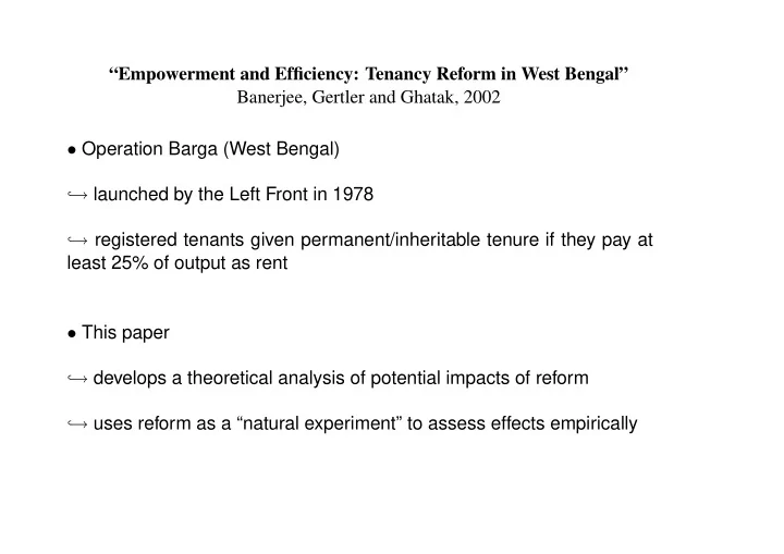
, launched by the Left Front in 1978 , registered tenants given - - PowerPoint PPT Presentation

“Empowerment and Efficiency: Tenancy Reform in West Bengal” Banerjee, Gertler and Ghatak, 2002

• Operation Barga (West Bengal)

, → launched by the Left Front in 1978 , → registered tenants given permanent/inheritable tenure if they pay at

least 25% of output as rent

• This paper

, → develops a theoretical analysis of potential impacts of reform , → uses reform as a “natural experiment” to assess effects empirically

The Theoretical Model Infinitely lived risk–neutral landlord Large population of infinitely–lived risk–neutral tenants with reservation payoff m per period Subjective discount factor δ Output:

y = ½

1 with probability e 0 with probability 1 − e where e is the tenant’s effort — non-observable Cost to tenant of supplying effort:

C(e) = c

2e2.

Limited liability: Tenants rent plus sharecropping payment is limited by his wealth, w Contract specifies:

h = payment to the tenant ϕ = probability of no eviction ¾

when y = 1

l = payment to the tenant ψ = probability of no eviction ¾

when y = 0

Optimal Tenancy Contracts without Eviction

, → one–period contracting problem

• Landord’s maximization problem

max

e,h,l

π = e − [eh + (1 − e)l] , → subject to h ≥ −(1 + w) and l ≥ −w

(LLC)

v = eh + (1 − e)l − c

2e2 ≥ m (PC)

e = argmax

e

n eh + (1 − e)l − c

2e2o (ICC)

• The ICC can be written as

e = h − l c , → note that it must be that h > l

• Substituting for e the problem becomes

max

h,l

π = h − l c − (h − l)2 c2 − l

subject to (h − l)2 2c + l ≥ m (PC)

l ≥ −w

(LLC)

• The value of e implied by the optimal contract:

e∗ =   

1/2c if m + w < 1/8c (LLC only binds)

p

2(m + w)/c if 1/8c ≤ m + w < 1/2c (both bind) 1/c if 1/2c ≤ m + w (PC only binds)

⇒ increase in outside option m (weakly) increases effort

(bargaining power effect)

l e

• w

A B C Increasing m 12.

empowerment and efficiency 249

• Fig. 1

Optimal Tenancy Contracts with Eviction

, → works like Shapiro–Stiglitz (1986), but with endogenous effort V = expected lifetime utility of an incumbent tenant M = m/(1 − δ) = expected lifetime utility of someone who is not a tenant

Assume the LLC binds (otherwise eviction has no effect)

• Expected lifetime utility from choosing e today:

V0 = max

e

n eh + δ [ϕe + (1 − e)ψ] (V − M) + δM − (1 − e)w − c

2e2o

, → the first–order condition yields h + w + δ (V − M) (ϕ − ψ) = cˆ e

• It is optimal for the landlord to set ϕ = 1 and ψ = 0. Why ?

, → and so h + w + δ (V − M) = cˆ e

(ICC)

• In a stationary equilibrium V0 = V and so expected Tenant utility is

V = ˆ eh + δˆ e (V − M) + δM − (1 − ˆ e)w − c

2ˆ

e2 , → this can be re-written as V − M = ˆ eh − (1 − ˆ e)w − c

2ˆ

e2 − m

1 − δˆ

e

(AB)

, → the stationary contract must offer this to be incentive compatible , → V − M is inceasing convex function of e, and decreasing in w and m

• The landlord’s problem is

max

e,h,l

e(1 − h) − (1 − e)l

subject to (ICC) and LLC (l = −w).

, → substituting these in we get

max

e

n e − c

2e2 + δ (V − M) e + w

• The FOC implies

e∗ = 1 + δ (V − M)

2c (CD)

, → the more surplus the Tenant gets, the more effort is required by the

Landlord

empowerment and efficiency 251

• Fig. 2

Broad Predictions of Theory

• Removing the threat of eviction weakens dynamic incentives to provide

effort

, → matters when m + w is low and LLC is binding

• BUT forbidding eviction increases Tenant’s outside option, m

, → increases the share of the output they receive , → increased effort

• also reduces incentive to make long–run investments

⇒ Trade-off between the dynamic and static incentive effects

256 journal of political economy

• Fig. 3.—Crop share of tenants before and after the reform

Implications of Operation Barga for Crop Shares

• Significant improvement in tenants’ contracts and more secure tenure
• Tenants receiving >50% of output rose from 17% to 39%
• 1977 — 1995, 30% of cultivated land was sold to sharecroppers

, → sharp contrast to other Indian states

empowerment and efficiency 259

• Fig. 4.—Rice yield in West Bengal and Bangladesh, 1969–93

TABLE 1 Summary Statistics

Log(Rice Yield, kg per Hectare) HYV Share,a 1977–93 (3) Proportion of Registered Tenants,b 1978–92 (4) Log(Area under Public Irri- gation, Hectare),c 1977–93 (5) Log(Road Length, km),d 1977–93 (6) Log(Rainfall, mm), 1977–93 (7) 1969–93 (1) 1977–93 (2) West Bengal (Annual Observations on 14 Districts) Grand mean 7.24 7.32 .11 .49 10.01 6.99 7.42 Standard deviation: Overall .31 .31 .09 .23 1.80 .39 .41 Within .23 .22 .05 .18 .30 .07 .24 Mean in: 1969 7.06 … … … … … … 1977 7.20 7.20 .06 … 9.91 6.93 7.24 1979 7.07 7.07 .06 .15 9.92 6.94 7.17 1993 7.60 7.60 .18 .65 10.13 7.02 7.58 Bangladesh (Annual Observations on 15 Districts) Grand mean 7.22 7.30 .15 11.36 … 7.69 Standard deviation: Overall .23 .20 .11 .89 … .35 Within .19 .15 .07 .43 … .21 Mean in: 1969 7.05 … … … … … … 1977 7.16 7.16 .09 11.00 … 7.62 1979 7.14 7.14 .09 11.06 … 7.64 1993 7.51 7.51 .25e 11.76 … 7.84

a Fraction of total rice area devoted to the cultivation of the summer crop, boro. b Registration data are relevant only for West Bengal and are available for the period 1978–93. c Public minor irrigation schemes include shallow tube wells, deep tube wells, and river lift irrigation. d This information is not available as a continuous series for Bangladesh during the period of analysis. e Information on HYV share for Bangladesh is available up to 1991, so this number pertains to 1991.

empowerment and efficiency 263

TABLE 2 Difference-in-Difference Models of Log of Rice Yield per Hectare (1969–93) Difference (1969–78) (1) Level 1969–93 (2) Excluding 1981–82 (3) West Bengal (p1) .004 (.17) … … West Bengal# (1979–83)a …

• .09***

(3.75) .01 (.38) West Bengal# (1984–88) … .05** (1.99) .05** (2.00) West Bengal# (1988–93) … .05* (1.77) .05* (1.78) District fixed effects F- statistic … 44.55 42.61 Year fixed ef- fects F- statistic 4.26*** 29.75*** 31.81***

2

R .12 .80 .81 Sample size 256 717 659

Note.—t-statistics are in parentheses.

a These variables are obtained by interacting a dummy variable that takes the value one if a district is in West Bengal

and zero if it is in Bangladesh with another dummy variable that takes the value one if the observation is in the indicated time period (1979–83 in this case) and zero otherwise. * Significant at the 10 percent level. ** Significant at the 5 percent level. *** Significant at the 1 percent level.

empowerment and efficiency 265

TABLE 3 Difference-in-Difference Models of Log of Rice Yield (1977–91)

Whole Sample Excluding Drought Years 1981–82 Model 1 Model 2 Model 3 Model 1 Model 2 Model 3 West Bengal# (1979–83) .08*** (2.43) .07** (2.05) .05 (1.58) .001 (.01) .002 (.06) .015 (.47) West Bengal# (1984–87) .04 (1.17) .05 (1.47) .07** (2.04) .04 (1.24) .04 (1.26) .06** (1.93) West Bengal# (1988–91) .08** (2.20) .12*** (3.28) .18*** (5.11) .07** (2.33) .11*** (2.97) .17*** (4.95) Log(rainfall) … .01 (.40) .007 (.32) … .019 (.70) .01 (.46) Log(public irrigation) … .122*** (7.22) .07*** (4.27) … .103 (5.77) .04*** (2.69) HYV share of grain cultivation area … … 1.04*** (8.18) … … 1.05*** (8.21) District fixed effects F-statistic 40.02*** 20.14*** 14.76*** 41.43*** 18.8*** 14.64*** Year fixed effects F-statistic 20.18*** 12.14*** 7.73*** 21.67*** 12.41*** 6.04***

2

R .82 .85 .87 .83 .85 .88 Sample size 424 424 424 367 367 367

Note.—t-statistics are in parentheses. ** Significant at the 5 percent level. *** Significant at the 1 percent level.

Empirical Results

• Between 1979 and 1993 rice yields in West Bengal rose by 69%,

compared to 44% in Bangladesh

• “Differences–in–differences” approach using districts in West Bengal

and Bangladesh ln ydt = αd + ψt + β × treamentd × postt +

X φjXjdt + ²dt∗ αd = district fixed effects ψt = year dummy

treatmentd = dummy for whether district is in West Bengal postt = post-reform year dummy

Xjdt = control variables , → β is the difference-indifference estimate of the impact of reform ⇒ Operation Barga accounted for 28% of additional growth