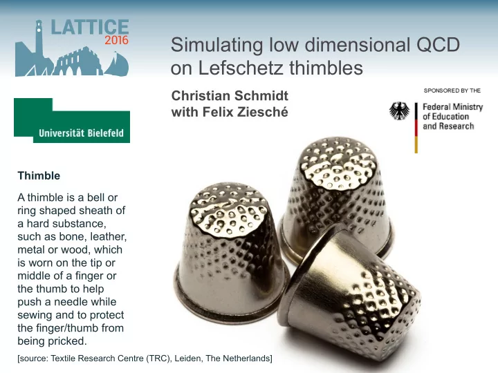

LATTICE Simulating low dimensional QCD 2016 on Lefschetz thimbles Christian Schmidt with Felix Ziesché Thimble A thimble is a bell or ring shaped sheath of a hard substance, such as bone, leather, metal or wood, which is worn on the tip or middle of a finger or the thumb to help push a needle while sewing and to protect the finger/thumb from being pricked. [source: Textile Research Centre (TRC), Leiden, The Netherlands]
Motivation: LATTICE 2016 The QCD sign problem The QCD partition function Z } e − S G [ U ] Z ( T, V, m, µ ) = D U det M [ U ] | {z complex for µ > 0 Lattice Dirac spectrum [det M ( µ )] ∗ = det M ( − µ ∗ ) 1. Barbour et al. / Simulations of lattice QCD 302 T > 0 T = 0 0.3 /d,a 4 3 × 8 • standard MC techniques not applicable 4 4 (a) • highly oscillatory integral with exponentially large cancellations *( Barbour et al. , 1986 Muroya et al. , 2003 I I 0.5 1.0 0.0 Re 5, C. Schmidt, Lattice 2016, Southampton, UK 2 /.La 0.6 (b) .< 0.0 0.5 1.0 Re 5, Fig. 2. The distribution of eigenvalues )t of the Dirac matrix for staggered fermions at fl = 0. Shown are the eigenvalues obtained from 6 random gauge configurations (fl = 0 quenched) on a 4 3 x g lattice for different values of the chemical potential, t* = 0.3 (a), 0,6 (b), 0.9 (c), and 1,2 (d).
Idea: LATTICE 2016 Deforming the domain of integration 0.6 Re[exp(-S)] along J 1 0.5 Standard 1d-example: the Airy integral numerical 0.4 integration Z ∞ ✓ x 3 1 ⇢ ◆� 0.3 Ai[1] = d x exp 3 + x easy! i 2 π −∞ 0.2 x → z = x + iy 0.1 6 0 J 1 z -6 -4 -2 0 2 4 6 real domain 4 Re[exp(-S)] along real domain 1 2 0 0.5 -2 0 -4 -0.5 -6 -1 -6 -4 -2 0 2 4 6 -6 -4 -2 0 2 4 6 numerical integration hopeless! see also Witten: 1001.2933, 1009.6032 C. Schmidt, Lattice 2016, Southampton, UK 3
Idea: LATTICE 2016 Deforming the domain of integration Standard 1d-example: the Airy integral Theory behind: Picard-Lefschetz theory • use the real valued function Z ∞ ✓ x 3 1 ⇢ ◆� S R ( z ) = Re[ − i ( z 3 / 3 + z )] Ai[1] = d x exp 3 + x i 2 π as a Morse function −∞ x → z = x + iy 6 J 1 z real domain 4 2 0 -2 -4 -6 -6 -4 -2 0 2 4 6 see also Witten: 1001.2933, 1009.6032 C. Schmidt, Lattice 2016, Southampton, UK 4
Idea: LATTICE 2016 Deforming the domain of integration Standard 1d-example: the Airy integral Theory behind: Picard-Lefschetz theory • use the real valued function Z ∞ ✓ x 3 1 ⇢ ◆� S R ( z ) = Re[ − i ( z 3 / 3 + z )] Ai[1] = d x exp 3 + x i 2 π as a Morse function −∞ x → z = x + iy • find all separated saddle points ( ) σ i 6 J 1 z real domain 4 2 σ 1 0 σ 2 -2 -4 -6 -6 -4 -2 0 2 4 6 see also Witten: 1001.2933, 1009.6032 C. Schmidt, Lattice 2016, Southampton, UK 5
Idea: LATTICE 2016 Deforming the domain of integration Standard 1d-example: the Airy integral Theory behind: Picard-Lefschetz theory • use the real valued function Z ∞ ✓ x 3 1 ⇢ ◆� S R ( z ) = Re[ − i ( z 3 / 3 + z )] Ai[1] = d x exp 3 + x i 2 π as a Morse function −∞ x → z = x + iy • find all separated saddle points ( ) σ i 6 • associated with each saddle point ( ), J 1 ,J 2 σ i z K 1 K 1 ,K 2 find one stable ( ) and one unstable J i real domain 4 J 1 thimble ( ) as solutions of the K i steepest descent/ascent flow equation 2 σ 1 d z (note: remains S I ( z ) 0 σ 2 d t = ⌥r S R ( z ) const. along flow) K 2 -2 -4 J 2 -6 -6 -4 -2 0 2 4 6 see also Witten: 1001.2933, 1009.6032 C. Schmidt, Lattice 2016, Southampton, UK 6
Idea: LATTICE 2016 Deforming the domain of integration Standard 1d-example: the Airy integral Theory behind: Picard-Lefschetz theory • use the real valued function Z ∞ ✓ x 3 1 ⇢ ◆� S R ( z ) = Re[ − i ( z 3 / 3 + z )] Ai[1] = d x exp 3 + x i 2 π as a Morse function −∞ x → z = x + iy • find all separated saddle points ( ) σ i 6 • associated with each saddle point ( ), J 1 ,J 2 σ i z K 1 K 1 ,K 2 find one stable ( ) and one unstable J i real domain 4 J 1 thimble ( ) as solutions of the K i steepest descent/ascent flow equation 2 σ 1 d z (note: remains S I ( z ) 0 σ 2 d t = ⌥r S R ( z ) const. along flow) K 2 -2 • decompose original integral into thimbles -4 J 2 Z Z d z e − S ( z ) = X n i e − S I ( σ i ) d z e − S R ( z ) -6 -6 -4 -2 0 2 4 6 R J i i (here: ) n 1 = 1 , n 2 = 0 , S I ( σ 1 ) = 0 see also Witten: 1001.2933, 1009.6032 C. Schmidt, Lattice 2016, Southampton, UK 7
Idea: LATTICE 2016 Deforming the domain of integration Original domain of integration real dim. 4 × V × 8 U x, ν ∈ SU(3) U 4 V ( ) X U = exp − i ω a T a a Complexified space ˜ real dim. U x, ν ∈ SL(3 , C ) 4 × V × 8 × 2 ˜ U 4 V New domain(s) of integration: Lefschetz thimble real dim. 4 × V × 8 J 0 + J 1 + · · · n ˜ U x, ν | U ( τ ) is solution of the SD equation with J 0 := o U (0) = ˜ and U ( τ → ∞ ) = N U x, ν here denotes the gauge orbit of the unity configuration N C. Schmidt, Lattice 2016, Southampton, UK 8
LATTICE Open questions: 2016 How many relevant thimbles are there in full QCD? How to sample them? • Langevin on the thimble (Aurora-algorithm) Cristoforetti et al., PRD 86 (2012) 074506 • HMC on the thimble Fujii et al., JHEP 1310 (2013) 147 • Use a map of the thimble (projection-, contraction-algorithm) A. Mukherjee et al., PRD 88 (2013) 051502; A. Alexandru et. al., PRD 93 (2016) 014504 • Sample SD paths on the thimble Di Renzo et al., PRD 88 (2013) 051502 C. Schmidt, Lattice 2016, Southampton, UK 9
LATTICE Open questions: 2016 How many relevant thimbles are there in full QCD? How to sample them? How to combine results from different thimbles? • input a number of physical quantities to determine relative weights Di Renzo et al., PRD 88 (2013) 051502 ⌦ e i φ O i ↵ ⌦ e i φ O i ↵ ⌦ e i φ O i ↵ α i = n i e S I ( σ i ) Z i 0 + α 1 1 + α 2 2 X i = i = 1 , 2 h e i φ i 0 + α 1 h e i φ i 1 + α 2 h e i φ i 2 , , n 0 e S I ( σ 0 ) Z 0 here denotes the residual phase (see ) φ Cristoforetti et al., PRD 89 (2014) 114505 C. Schmidt, Lattice 2016, Southampton, UK 10
LATTICE Open questions: 2016 How many relevant thimbles are there in full QCD? How to sample them? How to combine results from different thimbles? • input a number of physical quantities to determine relative weights • sample multiple thimbles at once, or one manifold that comes arbitrary close to multiple thimbles A. Alexandru et. al., JHEP 1605 (2016) 053 4 0.75 2 T = 0.5 0.70 � Im � T = 0.05 0 S R - 2 0.65 T = 0.01 - 4 0.60 - 1.5 - 1.0 - 0.5 0.0 0.5 1.0 1.5 - 1.0 - 0.5 0.0 0.5 1.0 � � ) far Re � Re ( � C. Schmidt, Lattice 2016, Southampton, UK 11
LATTICE Open questions: 2016 How many relevant thimbles are there in full QCD? How to sample them? How to combine results from different thimbles? How to deal with the gauge orbits? • perform simulations in a fixed gauge • make use of the gauge gauge transformations C. Schmidt, Lattice 2016, Southampton, UK 12
LATTICE Systems studied so far: 2016 φ 4 -theory Cristoforetti et al., PRD 88 (2013) 051501; Fujii et al., JHEP 1310 (2013) 147 Cristoforetti et al., PRD 89 (2014) 114505 Hubbard model, one-site Hubbard model A. Mukherjee et al., PRD 88 (2013) 051502 (0+1)dim. Thirring model Fujii et al., JHEP 1511 (2015) 078; Fujii et al., JHEP 1512 (2015) 125; Chiral random matrix model Di Renzo et al., PRD 88 (2013) 051502 . (also applications to QM-systems in real time) . . C. Schmidt, Lattice 2016, Southampton, UK 13
LATTICE Agenda: 2016 QCD in (0+1) dim. with std. staggered quarks • simulations in Polyakov loop diagonal form • simulations with a general Polyakov loop QCD in (n+1) dim. with std. staggered quarks • simulations at strong coupling • simulations away from strong coupling C. Schmidt, Lattice 2016, Southampton, UK 14
LATTICE Agenda: 2016 } QCD in (0+1) dim. with std. staggered quarks this talk :-) • simulations in Polyakov loop diagonal form • simulations with a general Polyakov loop } QCD in (n+1) dim. with std. staggered quark • simulations at strong coupling not yet :-( • simulations away from strong coupling C. Schmidt, Lattice 2016, Southampton, UK 15
LATTICE (0+1) dimensional QCD 2016 partition function in the reduced form Z Z ( N f ) = d P det N f [ A + e µ/T P + e − µ/T P − 1 ] | {z } D A = 2 cosh(ˆ µ c ) 1 3 Bilic et al. Phys. Lett. B212 (1988) 83 (see e.g. ) µ c = arcsinh( ˆ ˆ m ) Ammon et al., arXiv:1607.05027 diagonalize Polyakov loop P = diag( e i θ 1 , e i θ 2 , e − i ( θ 1 + θ 2 ) ) 8 ✓ 2 θ 1 + θ 2 ✓ θ 1 + 2 θ 2 ✓ θ 1 − θ 2 ◆ ◆ ◆ 3 π 2 sin 2 sin 2 sin 2 J ( θ 1 , θ 2 ) = 2 2 2 Z Z ( N f ) = d θ 1 d θ 2 e − S eff ( N f , θ 1 , θ 2 ) S eff = − (ln J + Tr ln D ) C. Schmidt, Lattice 2016, Southampton, UK 16
Recommend
More recommend