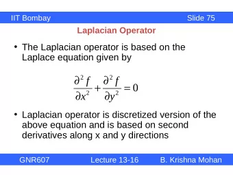
Laplacian approximation on graphs applied to signal and image - PowerPoint PPT Presentation
Laplacian approximation on graphs applied to signal and image restoration by Ph.D. Davide Bianchi Universit` a degli Studi dellInsubria Dip. di Scienze e Alta Tecnologia Como, 16 th of July 2018 1 of 30 Our model problem y = x +
Laplacian approximation on graphs applied to signal and image restoration by Ph.D. Davide Bianchi Universit` a degli Studi dell’Insubria Dip. di Scienze e Alta Tecnologia Como, 16 th of July 2018 1 of 30
Our model problem y δ = x ∗ + K noise • K represents the blur and it is severely ill-conditioned (compact integral operator of the first kind); • y δ are known measured data (blurred and noisy image); • � noise � ≤ δ . 2 of 30
Let’s reformulate the problem x ∈ R n � K x − y � 2 2 + α � x � 2 • Tikhonov: argmin 2 3 of 30
Let’s reformulate the problem x ∈ R n � K x − y � 2 2 + α � x � 2 • Tikhonov: argmin 2 x ∈ R n � K x − y � 2 2 + α � L x � 2 • Generalized Tikhonov: argmin 2 . L is semi-positive definite and ker( L ) ∩ ker( K ) = � 0 . ker( L ) should ‘ approximate the features ’of x † 3 of 30
Laplacian - Finite Difference approximation Poisson (Sturm-Liouville) problem on [0 , 1] : − ∆ x ( t ) = f ( t ) t ∈ (0 , 1) , α 1 x (0) + β 1 x ′ (0) = γ 1 , α 2 x (1) + β 2 x ′ (1) = γ 2 . If we consider Dirichlet homogeneous boundary conditions ( x (0) = x (1) = 0 ) and 3-point stencil FD approximation: − ∆ x ( t ) ≈ − x ( t − h ) + 2 x ( t ) − x ( t + h ) , h 2 = n − 2 , h 2 2 − 1 0 · · · − 1 2 − 1 · · · ker( L ) = � − L = 0 . ... ... ... 0 − 1 2 4 of 30
Laplacian - Finite Difference approximation · · · If we consider Neumann homogeneous boundary conditions ( x ′ (0) = x ′ (1) = 0 ) and 3-point stencil FD approximation: − ∆ x ( t ) ≈ − x ( t − h ) + 2 x ( t ) − x ( t + h ) , h 2 = n − 2 , h 2 1 − 1 0 · · · − 1 2 − 1 · · · ker( L ) = Span { � − L = 1 } . ... ... ... 0 − 1 1 5 of 30
An easy 1 d example of oversmoothing - part 2 Blur taken from Heat ( n, κ ) in Regtools , n = 100 , κ = 1 and 2% noise . True solution: � 0 if 0 ≤ t ≤ 0 . 5 , x † : [0 , 1] → R x † ( t ) = s.t. 1 if 0 . 5 < t ≤ 1 . 1.2 1 True solution Tik + L dirichlet 0.8 Tik + L neumann blurred&noisy signal 0.6 0.4 0.2 0 -0.2 0 0.1 0.2 0.3 0.4 0.5 0.6 0.7 0.8 0.9 1 6 of 30
Graph Laplacian • An image/signal x can be represented by a weighted undirected graph G = ( V, E, w ) : ◦ the nodes v i ∈ V are the pixels of the image/signal and x i ≥ 0 is the color intensity of x at v i . ◦ an edge e i,j ∈ E ⊆ V × V exists if the pixels v i and v j are connected, i.e., v i ∼ v j . ◦ w : E → R is a similarity (positive) weight function, w ( e i,j ) = w i,j . • The graph Laplacian is defined as � w i,j > 0 if v j ∼ v i , � − ∆ ( n ) w x i = w i,j ( x i − x j ) , w i,j = 0 otherwise. v j ∼ v i 7 of 30
Graph Laplacian - Example Example . In the 1 d case, if we define � 1 if v i ∼ v j , v i ∼ v j iff i = j + 1 or i = j − 1 , w i,j = 0 otherwise , then it holds 1 − 1 0 · · · − 1 2 − 1 · · · − ∆ ( n ) = L ( n ) = . ... ... ... w w 0 − 1 1 8 of 30
Question Why should the red points be connected? 1.2 1 0.8 0.6 0.4 0.2 0 -0.2 0 0.1 0.2 0.3 0.4 0.5 0.6 0.7 0.8 0.9 1 9 of 30
Answer They should not, indeed 1.2 1 true Tik + graph 0.8 0.6 0.4 0.2 0 -0.2 0 0.1 0.2 0.3 0.4 0.5 0.6 0.7 0.8 0.9 1 � � L ( n/ 2) 0 L ( n ) w = w L ( n/ 2) 0 w 10 of 30
Problems • Detection of the discontinuity points. 11 of 30
Problems • Detection of the discontinuity points. ◦ pre-denoising + first derivatives? 11 of 30
Problems • Detection of the discontinuity points. ◦ pre-denoising + first derivatives? • Choice of the weights w i,j . Indeed, for example another common choice of the weights is: � vi − vj � e − if � v i − v j � ≤ δ/ 2 , 2 σ 2 w i,j = 0 otherwise , 11 of 30
Problems • Detection of the discontinuity points. ◦ pre-denoising + first derivatives? • Choice of the weights w i,j . Indeed, for example another common choice of the weights is: � vi − vj � e − if � v i − v j � ≤ δ/ 2 , 2 σ 2 w i,j = 0 otherwise , ◦ finding the best weights that can approximate the Euclidean Laplacian. 11 of 30
Approximating the continuous Laplacian by graphs 1 − 1 0 · · · − 1 2 − 1 · · · � ( j − 1) π � � λ j ( L ( n ) − L ( n ) = ⇒ w ) = 2 sin ... ... ... w n 0 − 1 1 12 of 30
What does happen when we refine the grid? 13 of 30
FD approximation - 1/3 We have already highlighted that Finite Difference 3-point stencil ⇐ ⇒ graph-Laplacian Can we argue the same relationship if we use a wider stencil, i.e., if we ”connect” more points? 14 of 30
FD approximation - 2/3 Let us use a 5-point stencil. − ∆ x ( t ) ≈ x ( t − 2 h ) − 16 x ( t − h ) + 30 x ( t ) − 16 x ( t + h ) + x ( t − 2 h ) , 12 h 2 then 15 − 16 1 0 · · · 12 12 12 − 16 31 − 16 1 0 · · · 12 12 12 12 ... ... ... ... − L ( n ) = − L ( n ) = . w w 1 − 16 30 − 16 1 · · · · · · 12 12 12 12 12 ... ... 15 of 30
FD approximation 3/3 We have seen that negative weights appear. Does it make sense? • Does it approximate better the continuous Laplacian? Yes. • Is it still a graph-Laplacian? Yes. • Does it improve the reconstruction of our signal/image? Yes. 16 of 30
Spectral approximation 17 of 30
graph-Laplacian - distributional point of view − x ′′ ( t 0 ) = � x ′′ ( t ) , δ t 0 ( t ) � � + ∞ x ′′ ( t )sin(( t − t 0 ) πǫ − 1 ) = − lim dµ ( t ) π ( t − t 0 ) ǫ → 0 −∞ � + ∞ � ′′ � sin(( t − t 0 ) πǫ − 1 ) = − lim x ( t ) dµ ( t ) π ( t − t 0 ) ǫ → 0 −∞ ≈ − ( α − k x ( t 0 − kh ) + · · · + α 0 x ( t 0 ) + · · · + α k x ( t 0 − kh )) , where � ′′ � sin(( t − t 0 ) πǫ − 1 ) α j = µ ( I j ) · . π ( t − t 0 ) | t = t 0 + jh [ α − k · · · α − 1 α 0 α 1 · · · α k ] is our stencil for the Toeplitz. 18 of 30
Signed measures - 1/2 � ′′ � sin(( t − t 0 ) πǫ − 1 ) α j = µ ( I j ) · , π ( t − t 0 ) | t = t 0 + jh µ ( I j ) > 0 always � ′′ � sin(( t − t 0 ) πǫ − 1 ) changes sign . π ( t − t 0 ) | t = t 0 + jh Is it so dramatic that the sequence α j change signes? Remark The Lebesgue measure dµ ( · ) on [0 , 1] can be weakly approximated by a sequence of signed measures: n sin(( t − t k ) πn ) n →∞ n − 1 � dµ ( · ) = lim dµ ( · ) π ( t − t k ) k =1 19 of 30
Signed measures - 2/2 Fact: the spectrum of the graph-Laplacian that arises from FD schemes with increasing connected points, converges to the spectrum of the continuous Laplacian operator. The stencil converges to the Fourier coefficients of f ( θ ) = θ 2 : π 2 � − 1 1 1 − 1 � · · · − 2 − 2 4 · · · 4 2 3 2 20 of 30
The ’regularization parameter’ is the underlying geometry graph-Laplacian with 10 points connection and 2 connected components. No tuning of the regularization parameter α 21 of 30
Detection of the point of discontinuity 22 of 30
Example - deriv2 ( n, 3) , 2% noise 0 0 · · · · · · 0 π 2 / 3 − 2 − 2 1 / 2 · · · 0 � � L ( n/ 2) 0 ... ... ... ... L ( n ) w L ( n/ 2) = = w w L ( n/ 2) 0 w π 2 / 3 . . . 1 / 2 − 2 − 2 1 / 2 0 0 · · · · · · 0 0 ker( L ( n/ 2) ) = Span { � 1 ,� t } w 23 of 30
2D case - 5 point FD stencil example 0 . 0833 0 0 . 0833 0 0 . 0833 0 − 1 . 3333 − 1 . 3333 − 1 . 3333 0 0 . 0833 − 1 . 3333 10 − 1 . 3333 0 . 0833 0 − 1 . 3333 − 1 . 3333 − 1 . 3333 0 0 . 0833 0 0 . 0833 0 0 . 0833 24 of 30
2D example - denosing 1/2 25 of 30
2D example - denoising 2/2 26 of 30
2D example - Gaussian blur 27 of 30
Edge detection - 1/2 28 of 30
Edge detection - 2/2 29 of 30
Some references • Shuman, D. I., Narang, S. K., Frossard, P., Ortega, A., and Vandergheynst, P., The emerging field of signal processing on graphs: Extending high-dimensional data analysis to networks and other irregular domains , IEEE Signal Processing Magazine, 30(3), 83-98 (2013). • Faber, X. W. C., Spectral convergence of the discrete Laplacian on models of a metrized graph , New York J. Math, 12, 97-121 (2016). • Bianchi, D., and Donatelli, M., On generalized iterated Tikhonov regularization with operator-dependent seminorms , Electronic Transactions on Numerical Analysis, 47, 73-99 (2017). • Gerth, D., Klann, E., Ramlau, R., and Reichel, L., On fractional Tikhonov regularization. Journal of Inverse and Ill-posed Problems , 23(6), 611-625 (2008). • Bianchi, D., and Donatelli, M., Fractional-Tikhonov regularization on graphs for image restoration , preprint. 30 of 30
Recommend
More recommend
Explore More Topics
Stay informed with curated content and fresh updates.
