Language Models January 22, 2013 Tuesday, January 22, 13 Still no - PowerPoint PPT Presentation
Language Models January 22, 2013 Tuesday, January 22, 13 Still no MT?? Today we will talk about models of p (sentence) The rest of this semester will deal with p (translated sentence | input sentence) Why do it this way?
n -gram LMs p LM ( e ) = p ( e 1 , e 2 , e 3 , . . . , e ` ) p ( e 1 ) × ≈ p ( e 2 | e 1 ) × p ( e 3 | e 1 , e 2 ) × p ( e 4 | e 1 , e 2 , e 3 ) × · · · × p ( e ` | e 1 , e 2 , . . . , e ` − 2 , e ` − 1 ) Tuesday, January 22, 13
n -gram LMs p LM ( e ) = p ( e 1 , e 2 , e 3 , . . . , e ` ) p ( e 1 ) × ≈ p ( e 2 | e 1 ) × p ( e 3 | e 1 , e 2 ) × p ( e 4 | e 1 , e 2 , e 3 ) × · · · × p ( e ` | e 1 , e 2 , . . . , e ` − 2 , e ` − 1 ) Which do you think is better? Why? Tuesday, January 22, 13
n -gram LMs p LM ( e ) = p ( e 1 , e 2 , e 3 , . . . , e ` ) p ( e 1 ) × ≈ p ( e 2 | e 1 ) × p ( e 3 | e 1 , e 2 ) × p ( e 4 | e 1 , e 2 , e 3 ) × · · · × p ( e ` | e 1 , e 2 , . . . , e ` − 2 , e ` − 1 ) Tuesday, January 22, 13
n -gram LMs p LM ( e ) = p ( e 1 , e 2 , e 3 , . . . , e ` ) p ( e 1 ) × ≈ p ( e 2 | e 1 ) × p ( e 3 | e 1 , e 2 ) × p ( e 4 | e 1 , e 2 , e 3 ) × · · · × p ( e ` | e 1 , e 2 , . . . , e ` − 2 , e ` − 1 ) ` Y = p ( e 1 | START) × p ( e i | e i − 1 ) × p (STOP | e ` ) i =2 Tuesday, January 22, 13
START Tuesday, January 22, 13
START my p ( my | START ) Tuesday, January 22, 13
START my friends p ( my | START ) × p ( friends | my ) Tuesday, January 22, 13
START my friends call p ( my | START ) × p ( friends | my ) × p ( call | friends ) Tuesday, January 22, 13
START my friends call me p ( my | START ) × p ( friends | my ) × p ( call | friends ) × p ( me | call ) Tuesday, January 22, 13
START my friends call me Alex p ( my | START ) × p ( friends | my ) × p ( call | friends ) × p ( me | call ) × p ( Alex | me ) Tuesday, January 22, 13
START my friends call me Alex STOP p ( my | START ) × p ( friends | my ) × p ( call | friends ) × p ( me | call ) × p ( Alex | me ) × p ( STOP | Alex ) Tuesday, January 22, 13
START my friends call me Alex STOP p ( my | START ) × p ( friends | my ) × p ( call | friends ) × p ( me | call ) × p ( Alex | me ) × p ( STOP | Alex ) START my friends dub me Alex STOP p ( my | START ) × p ( friends | my ) × p ( dub | friends ) × p ( me | dub ) × p ( Alex | me ) × p ( STOP | Alex ) Tuesday, January 22, 13
START my friends call me Alex STOP p ( my | START ) × p ( friends | my ) × p ( call | friends ) × p ( me | call ) × p ( Alex | me ) × p ( STOP | Alex ) START my friends dub me Alex STOP p ( my | START ) × p ( friends | my ) × p ( dub | friends ) × p ( me | dub ) × p ( Alex | me ) × p ( STOP | Alex ) Tuesday, January 22, 13
START my friends call me Alex STOP p ( my | START ) × p ( friends | my ) × p ( call | friends ) × p ( me | call ) × p ( Alex | me ) × p ( STOP | Alex ) START my friends dub me Alex STOP p ( my | START ) × p ( friends | my ) × p ( dub | friends ) × p ( me | dub ) × p ( Alex | me ) × p ( STOP | Alex ) These sentences have many terms in common. Tuesday, January 22, 13
Categorical Distributions A categorical distribution characterizes a random event that can take on exactly one of K possible outcomes. ( nb . we often call these “multinomial distributions”) if x = 1 p 1 X p i = 1 if x = 2 p 2 i p ( x ) = p i ≥ 0 ∀ i . . . if x = K p K 0 otherwise Tuesday, January 22, 13
p ( · ) p Outcome the 0.3 and 0.1 said 0.04 says 0.004 of 0.12 why 0.008 Why 0.0007 restaurant 0.00009 destitute 0.00000064 Probability tables like this are the workhorses of language (and translation) modeling. Tuesday, January 22, 13
p ( · | some context) p ( · | other context) p p Outcome Outcome the 0.6 the 0.01 and 0.04 and 0.01 said 0.009 said 0.003 says 0.00001 says 0.009 of 0.1 of 0.002 why 0.1 why 0.003 Why 0.00008 Why 0.0006 restaurant 0.0000008 restaurant 0.2 destitute 0.00000064 destitute 0.1 Tuesday, January 22, 13
p ( · | some context) p ( · | in ) p ( · | other context) p ( · | the ) p p Outcome Outcome the 0.6 the 0.01 and 0.04 and 0.01 said 0.009 said 0.003 says 0.00001 says 0.009 of 0.1 of 0.002 why 0.1 why 0.003 Why 0.00008 Why 0.0006 restaurant 0.0000008 restaurant 0.2 destitute 0.00000064 destitute 0.1 Tuesday, January 22, 13
LM Evaluation • Extrinsic evaluation: build a new language model, use it for some task (MT, ASR, etc.) • Intrinsic: measure how good we are at modeling language We will use perplexity to evaluate models Given: w , p LM 1 | w | log 2 p LM ( w ) PPL = 2 0 ≤ PPL ≤ ∞ Tuesday, January 22, 13
Perplexity • Generally fairly good correlations with BLEU for n -gram models • Perplexity is a generalization of the notion of branching factor • How many choices do I have at each position? • State-of-the-art English LMs have PPL of ~100 word choices per position • A uniform LM has a perplexity of | Σ | • Humans do much better • ... and bad models can do even worse than uniform! Tuesday, January 22, 13
Whence parameters? Tuesday, January 22, 13
Whence parameters? Estimation. Tuesday, January 22, 13
p ( x | y ) = p ( x, y ) p ( y ) p MLE ( x ) = count( x ) ˆ N p MLE ( x, y ) = count( x, y ) ˆ N p MLE ( x | y ) = count( x, y ) N ˆ × count( y ) N = count( x, y ) count( y ) Tuesday, January 22, 13
p ( x | y ) = p ( x, y ) p ( y ) p MLE ( x ) = count( x ) ˆ N p MLE ( x, y ) = count( x, y ) ˆ N p MLE ( x | y ) = count( x, y ) N ˆ × count( y ) N = count( x, y ) count( y ) Tuesday, January 22, 13
p ( x | y ) = p ( x, y ) p ( y ) p MLE ( x ) = count( x ) ˆ N p MLE ( x, y ) = count( x, y ) ˆ N p MLE ( x | y ) = count( x, y ) N ˆ × count( y ) N = count( x, y ) count( y ) p MLE ( call | friends ) = count( friends call ) ˆ count( friends ) Tuesday, January 22, 13
MLE & Perplexity • What is the lowest (best) perplexity possible for your model class? • Compute the MLE! • Well, that’s easy... Tuesday, January 22, 13
START my friends call me Alex STOP p ( my | START ) × p ( friends | my ) × p ( call | friends ) × p ( me | call ) × p ( Alex | me ) × p ( STOP | Alex ) START my friends dub me Alex STOP p ( my | START ) × p ( friends | my ) × p ( dub | friends ) × p ( me | dub ) × p ( Alex | me ) × p ( STOP | Alex ) Tuesday, January 22, 13
START my friends call me Alex STOP p ( my | START ) × p ( friends | my ) × p ( call | friends ) × p ( me | call ) × p ( Alex | me ) × p ( STOP | Alex ) MLE START my friends dub me Alex STOP p ( my | START ) × p ( friends | my ) × p ( dub | friends ) × p ( me | dub ) × p ( Alex | me ) × p ( STOP | Alex ) MLE Tuesday, January 22, 13
START my friends call me Alex STOP p ( my | START ) × p ( friends | my ) × p ( call | friends ) × p ( me | call ) × p ( Alex | me ) × p ( STOP | Alex ) MLE -3.65172 START my friends dub me Alex STOP p ( my | START ) × p ( friends | my ) × p ( dub | friends ) × p ( me | dub ) × p ( Alex | me ) × p ( STOP | Alex ) MLE -3.65172 Tuesday, January 22, 13
START my friends call me Alex STOP p ( my | START ) × p ( friends | my ) × p ( call | friends ) × p ( me | call ) × p ( Alex | me ) × p ( STOP | Alex ) MLE -3.65172 -2.07101 START my friends dub me Alex STOP p ( my | START ) × p ( friends | my ) × p ( dub | friends ) × p ( me | dub ) × p ( Alex | me ) × p ( STOP | Alex ) MLE -3.65172 -2.07101 Tuesday, January 22, 13
START my friends call me Alex STOP p ( my | START ) × p ( friends | my ) × p ( call | friends ) × p ( me | call ) × p ( Alex | me ) × p ( STOP | Alex ) MLE -3.65172 -2.07101 -3.32231 START my friends dub me Alex STOP p ( my | START ) × p ( friends | my ) × p ( dub | friends ) × p ( me | dub ) × p ( Alex | me ) × p ( STOP | Alex ) MLE -3.65172 -2.07101 - ∞ Tuesday, January 22, 13
START my friends call me Alex STOP p ( my | START ) × p ( friends | my ) × p ( call | friends ) × p ( me | call ) × p ( Alex | me ) × p ( STOP | Alex ) MLE -3.65172 -2.07101 -3.32231 -0.271271 START my friends dub me Alex STOP p ( my | START ) × p ( friends | my ) × p ( dub | friends ) × p ( me | dub ) × p ( Alex | me ) × p ( STOP | Alex ) MLE -3.65172 -2.07101 - ∞ -2.54562 Tuesday, January 22, 13
START my friends call me Alex STOP p ( my | START ) × p ( friends | my ) × p ( call | friends ) × p ( me | call ) × p ( Alex | me ) × p ( STOP | Alex ) MLE -3.65172 -2.07101 -3.32231 -0.271271 -4.961 START my friends dub me Alex STOP p ( my | START ) × p ( friends | my ) × p ( dub | friends ) × p ( me | dub ) × p ( Alex | me ) × p ( STOP | Alex ) MLE -3.65172 -2.07101 - ∞ -2.54562 -4.961 Tuesday, January 22, 13
START my friends call me Alex STOP p ( my | START ) × p ( friends | my ) × p ( call | friends ) × p ( me | call ) × p ( Alex | me ) × p ( STOP | Alex ) MLE -3.65172 -2.07101 -3.32231 -0.271271 -4.961 -1.96773 START my friends dub me Alex STOP p ( my | START ) × p ( friends | my ) × p ( dub | friends ) × p ( me | dub ) × p ( Alex | me ) × p ( STOP | Alex ) MLE -3.65172 -2.07101 -1.96773 - ∞ -2.54562 -4.961 Tuesday, January 22, 13
START my friends call me Alex STOP p ( my | START ) × p ( friends | my ) × p ( call | friends ) × p ( me | call ) × p ( Alex | me ) × p ( STOP | Alex ) MLE -3.65172 -2.07101 -3.32231 -0.271271 -4.961 -1.96773 START my friends dub me Alex STOP p ( my | START ) × p ( friends | my ) × p ( dub | friends ) × p ( me | dub ) × p ( Alex | me ) × p ( STOP | Alex ) MLE -3.65172 -2.07101 -1.96773 - ∞ -2.54562 -4.961 MLE assigns probability zero to unseen events Tuesday, January 22, 13
Zeros • Two kinds of zero probs: • Sampling zeros : zeros in the MLE due to impoverished observations • Structural zeros : zeros that should be there. Do these really exist? • Just because you haven’t seen something, doesn’t mean it doesn’t exist. • In practice, we don’t like probability zero, even if there is an argument that it is a structural zero. Tuesday, January 22, 13
Zeros • Two kinds of zero probs: • Sampling zeros : zeros in the MLE due to impoverished observations • Structural zeros : zeros that should be there. Do these really exist? • Just because you haven’t seen something, doesn’t mean it doesn’t exist. • In practice, we don’t like probability zero, even if there is an argument that it is a structural zero. the a ’s are nearing the end of their lease in oakland Tuesday, January 22, 13
Smoothing Smoothing an refers to a family of estimation techniques that seek to model important general patterns in data while avoiding modeling noise or sampling artifacts. In particular, for language modeling, we seek p ( e ) > 0 ∀ e ∈ Σ ∗ We will assume that is known and finite. Σ Tuesday, January 22, 13
Add- Smoothing α p ∼ Dirichlet( α ) x i ∼ Categorical( p ) ∀ 1 ≤ i ≤ | x | Assuming this model, what is the most probable value of p , having observed training data x ? (bunch of calculus - read about it on Wikipedia) x = count( x ) + α x − 1 p ∗ ∀ α x > 1 N + P x 0 ( α x 0 − 1) Tuesday, January 22, 13
Add- Smoothing α • Simplest possible smoother • Surprisingly effective in many models • Does not work well for language models • There are procedures for dealing with 0 < alpha < 1 • When might these be useful? Tuesday, January 22, 13
Interpolation • “Mixture of MLEs” p ( dub | my friends ) = λ 3 ˆ ˆ p MLE ( dub | my friends ) + λ 2 ˆ p MLE ( dub | friends ) + λ 1 ˆ p MLE ( dub ) 1 + λ 0 | Σ | Tuesday, January 22, 13
Interpolation • “Mixture of MLEs” p ( dub | my friends ) = λ 3 ˆ ˆ p MLE ( dub | my friends ) + λ 2 ˆ p MLE ( dub | friends ) + λ 1 ˆ p MLE ( dub ) 1 + λ 0 | Σ | Where do the lambdas come from? Tuesday, January 22, 13
Discounting Discounting adjusts the frequencies of observed events downward to reserve probability for the things that have not been observed. Note only when f ( w 3 | w 1 , w 2 ) > 0 count( w 1 , w 2 , w 3 ) > 0 We introduce a discounted frequency : 0 ≤ f ∗ ( w 3 | w 1 , w 2 ) ≤ f ( w 3 | w 1 , w 2 ) The total discount is the zero-frequency probability: f ⇤ ( w 0 | w 1 , w 2 ) X λ ( w 1 , w 2 ) = 1 − w 0 Tuesday, January 22, 13
Back-off Recursive formulation of probability: ( f ∗ ( w 3 | w 1 , w 2 ) if f ∗ ( w 3 | w 1 , w 2 ) > 0 p BO ( w 3 | w 1 , w 2 ) = ˆ α w 1 ,w 2 × λ ( w 1 , w 2 ) × ˆ p BO ( w 3 | w 1 , w 2 ) otherwise Tuesday, January 22, 13
Back-off Recursive formulation of probability: ( f ∗ ( w 3 | w 1 , w 2 ) if f ∗ ( w 3 | w 1 , w 2 ) > 0 p BO ( w 3 | w 1 , w 2 ) = ˆ α w 1 ,w 2 × λ ( w 1 , w 2 ) × ˆ p BO ( w 3 | w 1 , w 2 ) otherwise { “Back-off weight” Tuesday, January 22, 13
Back-off Recursive formulation of probability: ( f ∗ ( w 3 | w 1 , w 2 ) if f ∗ ( w 3 | w 1 , w 2 ) > 0 p BO ( w 3 | w 1 , w 2 ) = ˆ α w 1 ,w 2 × λ ( w 1 , w 2 ) × ˆ p BO ( w 3 | w 1 , w 2 ) otherwise { “Back-off weight” Question: how do we discount? Tuesday, January 22, 13
Witten-Bell Discounting Let’s assume that the probability of a zero off can be estimated as follows: λ ( a , b ) ∝ Tuesday, January 22, 13
Witten-Bell Discounting Let’s assume that the probability of a zero off can be estimated as follows: a λ ( a , b ) ∝ Tuesday, January 22, 13
Witten-Bell Discounting Let’s assume that the probability of a zero off can be estimated as follows: a b λ ( a , b ) ∝ Tuesday, January 22, 13
Witten-Bell Discounting Let’s assume that the probability of a zero off can be estimated as follows: a b c 1 λ ( a , b ) ∝ Tuesday, January 22, 13
Witten-Bell Discounting Let’s assume that the probability of a zero off can be estimated as follows: a b c a 1 λ ( a , b ) ∝ Tuesday, January 22, 13
Witten-Bell Discounting Let’s assume that the probability of a zero off can be estimated as follows: a b c a b 1 λ ( a , b ) ∝ Tuesday, January 22, 13
Witten-Bell Discounting Let’s assume that the probability of a zero off can be estimated as follows: a b c a b c 1 λ ( a , b ) ∝ Tuesday, January 22, 13
Witten-Bell Discounting Let’s assume that the probability of a zero off can be estimated as follows: a b c a b c a 1 λ ( a , b ) ∝ Tuesday, January 22, 13
Witten-Bell Discounting Let’s assume that the probability of a zero off can be estimated as follows: a b c a b c a b 1 λ ( a , b ) ∝ Tuesday, January 22, 13
Witten-Bell Discounting Let’s assume that the probability of a zero off can be estimated as follows: a b c a b c a b x 1+1 λ ( a , b ) ∝ Tuesday, January 22, 13
Witten-Bell Discounting Let’s assume that the probability of a zero off can be estimated as follows: a b c a b c a b x a 1+1 λ ( a , b ) ∝ Tuesday, January 22, 13
Witten-Bell Discounting Let’s assume that the probability of a zero off can be estimated as follows: a b c a b c a b x a b 1+1 λ ( a , b ) ∝ Tuesday, January 22, 13
Witten-Bell Discounting Let’s assume that the probability of a zero off can be estimated as follows: a b c a b c a b x a b c 1+1 λ ( a , b ) ∝ Tuesday, January 22, 13
Witten-Bell Discounting Let’s assume that the probability of a zero off can be estimated as follows: a b c a b c a b x a b c c 1+1 λ ( a , b ) ∝ Tuesday, January 22, 13
Witten-Bell Discounting Let’s assume that the probability of a zero off can be estimated as follows: a b c a b c a b x a b c c a 1+1 λ ( a , b ) ∝ Tuesday, January 22, 13
Witten-Bell Discounting Let’s assume that the probability of a zero off can be estimated as follows: a b c a b c a b x a b c c a b 1+1 λ ( a , b ) ∝ Tuesday, January 22, 13
Witten-Bell Discounting Let’s assume that the probability of a zero off can be estimated as follows: a b c a b c a b x a b c c a b a 1+1+1 λ ( a , b ) ∝ Tuesday, January 22, 13
Witten-Bell Discounting Let’s assume that the probability of a zero off can be estimated as follows: a b c a b c a b x a b c c a b a b 1+1+1 λ ( a , b ) ∝ Tuesday, January 22, 13
Witten-Bell Discounting Let’s assume that the probability of a zero off can be estimated as follows: a b c a b c a b x a b c c a b a b x 1+1+1 λ ( a , b ) ∝ Tuesday, January 22, 13
Witten-Bell Discounting Let’s assume that the probability of a zero off can be estimated as follows: a b c a b c a b x a b c c a b a b x c 1+1+1 λ ( a , b ) ∝ Tuesday, January 22, 13
Witten-Bell Discounting Let’s assume that the probability of a zero off can be estimated as follows: a b c a b c a b x a b c c a b a b x c 1+1+1 =3 λ ( a , b ) ∝ Tuesday, January 22, 13
Witten-Bell Discounting Let’s assume that the probability of a zero off can be estimated as follows: a b c a b c a b x a b c c a b a b x c 1+1+1 =3 λ ( a , b ) ∝ t ( a , b ) = |{ x : count( a , b , x ) > 0 }| Tuesday, January 22, 13
Witten-Bell Discounting Let’s assume that the probability of a zero off can be estimated as follows: a b c a b c a b x a b c c a b a b x c 1+1+1 =3 λ ( a , b ) ∝ t ( a , b ) = |{ x : count( a , b , x ) > 0 }| t ( a , b ) λ ( a , b ) = count( a , b ) + t ( a , b ) Tuesday, January 22, 13
Witten-Bell Discounting Let’s assume that the probability of a zero off can be estimated as follows: a b c a b c a b x a b c c a b a b x c 1+1+1 =3 λ ( a , b ) ∝ t ( a , b ) = |{ x : count( a , b , x ) > 0 }| t ( a , b ) λ ( a , b ) = count( a , b ) + t ( a , b ) count( a , b , c ) f ∗ ( c | a , b ) = count( a , b ) + t ( a , b ) Tuesday, January 22, 13
Kneser-Ney Discounting • State-of-the-art in language modeling for 15 years • Two major intuitions • Some contexts have lots of new words • Some words appear in lots of contexts • Procedure • Only register a lower-order count the first time it is seen in a backoff context • Example: bigram model • “San Francisco” is a common bigram • But, we only count the unigram “Francisco” the first time we see the bigram “San Francisco” - we change its unigram probability Tuesday, January 22, 13
Kneser-Ney II f ∗ ( b | a ) = max { t ( · , a , b ) − d, 0 } t ( · , a , · ) t ( · , a , b ) = |{ w : count( w, a , b ) > 0 }| t ( · , a , · ) = |{ ( w, w 0 ) : count( w, a , w 0 ) > 0 }| Tuesday, January 22, 13
Kneser-Ney II f ∗ ( b | a ) = max { t ( · , a , b ) − d, 0 } t ( · , a , · ) t ( · , a , b ) = |{ w : count( w, a , b ) > 0 }| t ( · , a , · ) = |{ ( w, w 0 ) : count( w, a , w 0 ) > 0 }| Max-order n-grams estimated normally! Tuesday, January 22, 13
Recommend
More recommend
Explore More Topics
Stay informed with curated content and fresh updates.

