Kalman Filter State Space Model Review Derivation x n +1 = F n x n - PowerPoint PPT Presentation

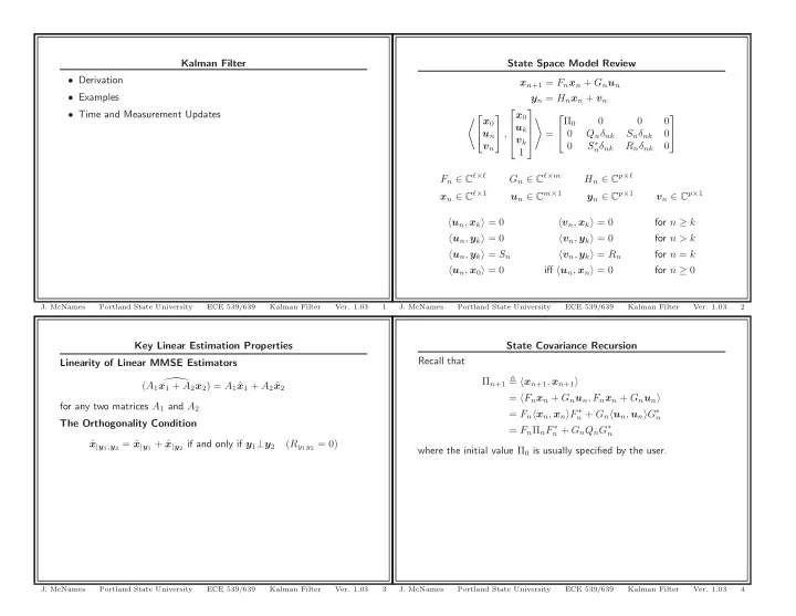
Kalman Filter State Space Model Review • Derivation x n +1 = F n x n + G n u n • Examples y n = H n x n + v n ⎡ ⎤ • Time and Measurement Updates x 0 �⎡ ⎤ ⎡ ⎤ Π 0 0 0 0 � x 0 u k ⎦ , ⎢ ⎥ = 0 Q n δ nk S n δ nk 0 u n ⎣ ⎢ ⎥ ⎣ ⎦ v k ⎣ ⎦ S ∗ 0 n δ nk R n δ nk 0 v n 1 F n ∈ C ℓ × ℓ G n ∈ C ℓ × m H n ∈ C p × ℓ x n ∈ C ℓ × 1 u n ∈ C m × 1 y n ∈ C p × 1 v n ∈ C p × 1 � u n , x k � = 0 � v n , x k � = 0 for n ≥ k � u n , y k � = 0 � v n , y k � = 0 for n > k � u n , y k � = S n � v n , y k � = R n for n = k � u n , x 0 � = 0 iff � u n , x n � = 0 for n ≥ 0 J. McNames Portland State University ECE 539/639 Kalman Filter Ver. 1.03 1 J. McNames Portland State University ECE 539/639 Kalman Filter Ver. 1.03 2 Key Linear Estimation Properties State Covariance Recursion Recall that Linearity of Linear MMSE Estimators Π n +1 � � x n +1 , x n +1 � � ( A 1 x 1 + A 2 x 2 ) = A 1 ˆ x 1 + A 2 ˆ x 2 = � F n x n + G n u n , F n x n + G n u n � for any two matrices A 1 and A 2 = F n � x n , x n � F ∗ n + G n � u n , u n � G ∗ n The Orthogonality Condition = F n Π n F ∗ n + G n Q n G ∗ n x | y 1 , y 2 = ˆ ˆ x | y 1 + ˆ x | y 2 if and only if y 1 ⊥ y 2 ( R y 1 y 2 = 0) where the initial value Π 0 is usually specified by the user. J. McNames Portland State University ECE 539/639 Kalman Filter Ver. 1.03 3 J. McNames Portland State University ECE 539/639 Kalman Filter Ver. 1.03 4

Innovations Recursion for Innovations Let us begin by just using the linear process model and the definition e n � y n − ˆ y n | n − 1 of the innovations y n = H n x n + v n e n � y n − ˆ y n = H n x n + v n y n | n − 1 y n | n − 1 = H n ˆ ˆ x n | n − 1 + ˆ v n | n − 1 • The estimator notation used here is = H n ˆ x n | n − 1 e n = y n − H n ˆ y n | k = the linear MMSE estimator of y n given { y 0 , . . . , y k } ˆ x n | n − 1 = H n x n + v n − H n ˆ x n | n − 1 • Our goal is to come up with a recursive formulation for linear = H n ( x n − ˆ x n | n − 1 ) + v n estimators of x n for n = 0 , 1 , . . . = H n ˜ x n | n − 1 + v n • Our motivation for using the innovations is that they have a diagonal covariance matrix where the new notation is defined as • Recall that calculating the innovations is equivalent to applying a x n | n − 1 � x n − ˆ ˜ y n | n − 1 � y n − ˆ ˜ y n | n − 1 = e n x n | n − 1 whitening filter – This has become a theme for this class Note that our goal of finding an expression for the innovations reduces – “Whiten before processing” to finding a way to estimate the one-step predictions of the state vector, ˆ – Simplifies the subsequent step of estimation x n | n − 1 J. McNames Portland State University ECE 539/639 Kalman Filter Ver. 1.03 5 J. McNames Portland State University ECE 539/639 Kalman Filter Ver. 1.03 6 State Estimation for Innovations State Estimation for Innovations x n +1 | n = � x n +1 , col { y 0 , . . . , y n }� � col { y 0 , . . . , y n }� − 2 col { y 0 , . . . , y n } n ˆ � � x n +1 , e k � R − 1 x n +1 | n = ˆ e,k e k = � x n +1 , col { e 0 , . . . , e n }� � col { e 0 , . . . , e n }� − 2 col { e 0 , . . . , e n } k =0 n • This expression assumes the error covariance matrix is invertible � � x n +1 , e k � R − 1 = e,k e k (positive definite) k =0 R e,k > 0 where we have defined • This is a nondegeneracy assumption on the process R e,k � � e k � 2 = E [ e k e ∗ k ] { y 0 , . . . , y n } • It essentially means that no variable y n can be exactly estimated • The first equality is just the solution to the normal equations by a linear combination of earlier observations • The second equality follows from the definition of the innovations • This does not require that R n = � v n � 2 > 0 and equivalence of the linear spaces spanned by the observations and innovations – It’s quite possible that R e,k > 0 even if R n = 0 L{ y 0 , . . . , y n } = L{ e 0 , . . . , e n } • However, if R n > 0 , we know for certain that R e,k > 0 • The third equality follows from the orthogonality property J. McNames Portland State University ECE 539/639 Kalman Filter Ver. 1.03 7 J. McNames Portland State University ECE 539/639 Kalman Filter Ver. 1.03 8

Circular Reasoning? Recursive State Estimation In order to calculate the innovations n � � x n +1 , e k � R − 1 x n +1 | n = ˆ e,k e k e n � y n − ˆ y n | n − 1 = y n − H n ˆ x n | n − 1 k =0 � n − 1 � we need to estimate the one step predictions of the state. Yet in order � � x n +1 , e k � R − 1 + � x n +1 , e n � R − 1 = e,k e k e,n e n to obtain these estimates, k =0 n x n +1 | n − 1 + � x n +1 , e n � R − 1 = ˆ � y n − H n ˆ � x n | n − 1 � e,n � x n +1 , e k � R − 1 x n +1 | n = ˆ e,k e k • This is almost what we need k =0 • However, there are still some missing pieces we need the innovations! – Can we express ˆ x n +1 | n − 1 in terms of what is known at time n : • Luckily, we only need the previous innovations to estimate the one x n | n − 1 and e n ? ˆ step state predictions – How do we obtain an expression for the error covariance matrix • Suggests a recursive solution in terms of the model parameters? • The only way to make any further progress is to use the state update equation that relates x n +1 to x n J. McNames Portland State University ECE 539/639 Kalman Filter Ver. 1.03 9 J. McNames Portland State University ECE 539/639 Kalman Filter Ver. 1.03 10 State Prediction Defining the State Error Covariance x n +1 = F n x n + G n u n x n | n − 1 � x n − ˆ ˜ x n | n − 1 x n +1 | n − 1 = F n ˆ ˆ x n | n − 1 + G n ˆ u n | n − 1 = F n ˆ x n | n − 1 x n | n − 1 � 2 = E � � P n | n − 1 � � ˜ x ∗ x n | n − 1 ˜ ˜ n | n − 1 Now given • We still need to solve for K p ,n and R e,n in terms of the known x n +1 | n − 1 + � x n +1 , e n � R − 1 � � x n +1 | n = ˆ ˆ y n − H n ˆ x n | n − 1 e,n state space model parameters we can set up a proper recursion that we initialize with e 0 = y 0 • To do so it will be useful to introduce yet another covariance e n = y n − H n ˆ matrix x n | n − 1 x n +1 | n = F n ˆ ˆ x n | n − 1 + K p ,n e n • P n | n − 1 is the state error covariance matrix where we have defined • It would be great to know this anyway K p ,n � � x n +1 , e n � R − 1 – Gives us a means of knowing how accurate our estimates are e,n – If { x 0 , u 0 , . . . , u n , v 0 , . . . , v n } are jointly Gaussian (central • The subscript p indicates that this gain is used to update a limit theorem) we could construct exact confidence intervals on predicted estimator of the state, ˆ x n +1 | n our estimates! • This is one of the Kalman gains that we will use J. McNames Portland State University ECE 539/639 Kalman Filter Ver. 1.03 11 J. McNames Portland State University ECE 539/639 Kalman Filter Ver. 1.03 12