Extended Kalman Filter Nonlinear State Space Model Derivation - PowerPoint PPT Presentation

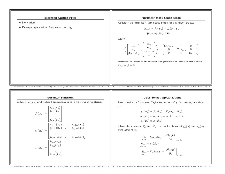
Extended Kalman Filter Nonlinear State Space Model • Derivation Consider the nonlinear state-space model of a random process • Example application: frequency tracking x n +1 = f n ( x n ) + g n ( x n ) u n y n = h n ( x n ) + v n where ⎡ ⎤ u m �⎡ ⎤ ⎡ ⎤ � Q n δ n,m 0 0 0 u n v m ⎢ ⎥ ⎦ , v n = 0 R n δ n,m 0 0 ⎢ ⎥ ⎣ ⎣ ⎦ x 0 − ¯ x 0 ⎣ ⎦ x 0 − ¯ x 0 0 0 Π 0 0 1 Assumes no interaction between the process and measurement noise, � u n , v m � = 0 J. McNames Portland State University ECE 539/639 Extended Kalman Filter Ver. 1.02 1 J. McNames Portland State University ECE 539/639 Extended Kalman Filter Ver. 1.02 2 Nonlinear Functions Taylor Series Approximations f n ( x n ) , g n ( x n ) and h n ( x n ) are multivariate, time-varying functions. Now consider a first-order Taylor expansion of f n ( x ) and h n ( x ) about x n . ˆ ⎡ ⎤ f n, 1 ( x n ) f n, 2 ( x n ) ⎢ ⎥ f n ( x n ) ≈ f n (ˆ x n ) + F n ( x n − ˆ x n ) ⎢ ⎥ f n ( x n ) = . ⎢ . ⎥ . h n ( x n ) ≈ h n (ˆ x n ) + H n ( x n − ˆ x n ) ⎣ ⎦ f n,k ( x n ) g n ( x n ) ≈ g n (ˆ x n ) ⎡ ⎤ g n, 11 ( x n ) . . . g n, 1 m ( x n ) where the matrices F n and H n are the Jacobians of f n ( x ) and h n ( x ) g n, 21 ( x n ) g n, 2 m ( x n ) . . . ⎢ ⎥ evaluated at ˆ x n ⎢ ⎥ g n ( x n ) = . . ... ⎢ . . ⎥ . . ⎣ ⎦ � = ∇ x f n ( x ) = ∂f n ( x ) � g n,ℓm ( x n ) . . . g n,ℓm ( x n ) F n � ∂ x � ℓ × ℓ ⎡ ⎤ x =ˆ x n h n, 1 ( x n ) m × m = g n (ˆ x n ) G n h n, 2 ( x n ) ⎢ ⎥ ⎢ ⎥ h n ( x n ) = . � ⎢ . ⎥ p × p = ∇ x h n ( x ) = ∂h n ( x ) � . ⎣ ⎦ H n � ∂ x h n,m ( x n ) � x =ˆ x n J. McNames Portland State University ECE 539/639 Extended Kalman Filter Ver. 1.02 3 J. McNames Portland State University ECE 539/639 Extended Kalman Filter Ver. 1.02 4

Taylor Series Approximations: Linearization Point Jacobians In expanded form, the Jacobians are given as follows • Taylor series expansion could be about different estimates of x n for each of the three nonlinear functions ⎡ ⎤ ∂f n, 1 ( x ) ∂f n, 1 ( x ) ∂f n, 1 ( x ) . . . ∂ x (1) ∂ x (2) ∂ x ( ℓ ) – ˆ x n | n is usually used for f n ( · ) and g n ( · ) ⎢ ⎥ ∂f n, 2 ( x ) ∂f n, 2 ( x ) ∂f n, 2 ( x ) . . . ⎢ ⎥ ∇ x f n ( x ) = ∂f n ( x ) ∂ x (1) ∂ x (2) ∂ x ( ℓ ) – ˆ x n | n − 1 is usually used for h n ( · ) ⎢ ⎥ = . . . ... ⎢ ⎥ ∂ x . . . ⎢ . . . ⎥ – The best possible estimate should be used in all cases to ⎣ ⎦ ∂f n,ℓ ( x ) ∂f n,ℓ ( x ) ∂f n,ℓ ( x ) minimize the error in the Taylor series approximations . . . ∂ x (1) ∂ x (2) ∂ x ( ℓ ) • Note that, even if the estimates ˆ x n and ˆ y n − 1 are unbiased, the ⎡ ∂h n, 1 ( x ) ∂h n, 1 ( x ) ∂h n, 1 ( x ) ⎤ . . . ∂ x (1) ∂ x (2) ∂ x ( ℓ ) estimates ˆ x n +1 | n and ˆ y n | n − 1 will be biased ∂h n, 2 ( x ) ∂h n, 2 ( x ) ∂h n, 2 ( x ) ⎢ ⎥ . . . ∇ x h n ( x ) = ∂h n ( x ) ⎢ ⎥ ∂ x (1) ∂ x (2) ∂ x ( ℓ ) = ⎢ ⎥ . . . ... ∂ x . . . ⎢ ⎥ . . . ⎣ ⎦ ∂h n,p ( x ) ∂h n,p ( x ) ∂h n,p ( x ) . . . ∂ x (1) ∂ x (2) ∂ x ( ℓ ) J. McNames Portland State University ECE 539/639 Extended Kalman Filter Ver. 1.02 5 J. McNames Portland State University ECE 539/639 Extended Kalman Filter Ver. 1.02 6 Affine State Space Approximation Accounting for the Nonzero Mean x n +1 ≈ f n (ˆ x n ) + F n ( x n − ˆ x n ) + G n u n x n +1 ≈ f n (ˆ x n ) + F n ( x n − ˆ x n ) + G n u n = F n x n + f n (ˆ x n ) − F n ˆ y n ≈ h n (ˆ x n ) + H n ( x n − ˆ x n + G n u n x n ) + v n � �� � Requires estimation • The Taylor series approximation results in an affine model y n ≈ h n (ˆ x n ) + H n ( x n − ˆ x n ) + v n • There are two key differences between this model and the linear = H n x n + ( h n (ˆ x n ) − H n ˆ x n ) + v n model � �� � – x n and y n have nonzero means Requires estimation – The coefficients are now random variables — not constants • The performance of the extended Kalman filter depends most critically on the accuracy of the Taylor series approximations • The typical approach to converting this to our linear model is to subtract the means from both sides • Most accurate when the state residual ( x n − ˆ x n ) is minimized • The EKF simply uses the best estimates that are available at the time that the residuals must be calculated J. McNames Portland State University ECE 539/639 Extended Kalman Filter Ver. 1.02 7 J. McNames Portland State University ECE 539/639 Extended Kalman Filter Ver. 1.02 8

Redefining the Normal Equations Centering the Output Equation The optimal estimate of the state is now defined as the optimal affine E[ y n ] = E[ h n (ˆ x n )] + H n (E[ x n ] − E[ˆ x n ]) + E[ v n ] transformation of y n = E[ h n (ˆ x n )] + H n (E[ x n ] − E[ˆ x n ]) x n +1 | n � K o y n + k = K o ( y n − E[ y n ]) + E[ x n +1 ] ˆ Now if we assume that ˆ x n is nearly deterministic (in other words, perfect) then In terms of the normal equations we have E[ˆ x n ] ≈ ˆ E[ h n (ˆ x n )] ≈ h n (ˆ x n ) x n +1 | n = � x n +1 , col { 1 , y 0 , . . . , y n }� � col { 1 , y 0 , . . . , y n }� − 2 col { 1 , y 0 , . . . , y n } x n ˆ = � x n +1 , col { 1 , e 0 , . . . , e n }� � col { 1 , e 0 , . . . , e n }� − 2 col { 1 , e 0 , . . . , e n } and this simplifies to n E[ y n ] ≈ h n (ˆ x n ) + H n (E[ x n ] − ˆ x n ) � x n +1 , e k � R − 1 � = µ n +1 + e,k e k Then the centered output is given by k =0 where the first innovation is now defined as y c ,n � y n − E[ y n ] e 0 � y 0 − ˆ ≈ [ h n (ˆ x n ) + H n ( x n − ˆ x n ) + v n ] − [ h n (ˆ x n ) + H n (E[ x n ] − ˆ x n )] y 0 = y 0 − E[ y 0 ] = H n ( x n − E[ x n ]) + v n + ( h n (ˆ x n ) − h n (ˆ x n )) + H n (ˆ x n − ˆ x n ) and all the innovations have zero mean by definition = H n x c ,n + v n J. McNames Portland State University ECE 539/639 Extended Kalman Filter Ver. 1.02 9 J. McNames Portland State University ECE 539/639 Extended Kalman Filter Ver. 1.02 10 State Mean Centering the State The expected value of x n +1 is µ n +1 = F n ( µ n − ˆ x n ) + f n (ˆ x n ) E[ x n +1 ] = F n E[ x n ] + E[ f n (ˆ x n )] − F n E[ˆ x n ] + G n E[ u n ] x c ,n +1 � x n +1 − µ n +1 µ n +1 = F n µ n + E[ f n (ˆ x n )] − F n E[ˆ x n ] = ( F n x n + f n (ˆ x n ) − F n ˆ x n + G n u n ) − ( F n µ n + f n (ˆ x n ) − F n ˆ x n ) = F n ( µ n − E[ˆ x n ]) + E[ f n (ˆ x n )] = F n ( x n − µ n ) + ( f n (ˆ x n ) − f n (ˆ x n )) − F n (ˆ x n − ˆ x n ) + G n u n Thus we obtain a recursive update equation for the state mean. Again, = F n x c ,n + G n u n if we assume that ˆ x n is nearly deterministic Thus our complete linearized state space model becomes E[ˆ x n ] ≈ ˆ x n E[ f n (ˆ x n )] ≈ f n (ˆ x n ) x c ,n +1 = F n x c ,n + G n u n The mean recursion then simplifies to y c ,n = H n x c ,n + v n µ n +1 = F n ( µ n − ˆ x n ) + f n (ˆ x n ) J. McNames Portland State University ECE 539/639 Extended Kalman Filter Ver. 1.02 11 J. McNames Portland State University ECE 539/639 Extended Kalman Filter Ver. 1.02 12

Linearization Points Estimating the State x n +1 ≈ f n (ˆ x n ) + F n ( x n − ˆ x n ) + G n u n x c ,n +1 = F n x c ,n + G n u n y n ≈ h n (ˆ x n ) + H n ( x n − ˆ x n ) + v n y c ,n = H n x c ,n + v n • The KF recursions will give us the optimal estimated state for the linearized model, ˆ x c ,n | n − 1 and ˆ x c ,n | n x n � ˆ • Best estimate of x n for the state prediction is ˆ x n | n • Conversion to the state estimates requires estimation of the state • Cannot be used for the output estimate because the innovation mean e n = y n − ˆ y n is required to calculate ˆ x n | n x n | n − 1 = ˆ ˆ x c ,n | n − 1 + µ n x n � ˆ • Thus, ˆ x n | n − 1 is used for the output linearization point x n | n = ˆ ˆ x c ,n | n + µ n • These estimates result in several simplifications • Would be convenient if we could estimate the state directly J. McNames Portland State University ECE 539/639 Extended Kalman Filter Ver. 1.02 13 J. McNames Portland State University ECE 539/639 Extended Kalman Filter Ver. 1.02 14 Predicted State Recursions Filtered State Recursions � � x n | n = ˆ ˆ x c ,n | n + µ n µ n − ˆ + f n (ˆ µ n +1 = F n x n | n x n | n ) � ˆ � x n +1 | n = ˆ ˆ x c ,n +1 | n + µ n +1 = x c ,n | n − 1 + K f ,n e n + µ n � � � � � � � ˆ � = F n ˆ + µ n − ˆ + f n (ˆ x n | n ) = x c ,n | n − 1 + µ n + K f ,n e n x c ,n | n F n x n | n = F n (ˆ x c ,n | n + µ n ) − F n ˆ x n | n + f n (ˆ x n | n ) = ˆ x n | n − 1 + K f ,n e n = F n ˆ x n | n − F n ˆ x n | n + f n (ˆ x n | n ) Thus the measurement updates can also be obtained directly in terms = f n (ˆ x n | n ) of the estimated state without having to estimate the state mean! Thus the time update can be obtained directly in terms of the estimated state without having to estimate the mean! x n +1 | n = f n (ˆ ˆ x n | n ) J. McNames Portland State University ECE 539/639 Extended Kalman Filter Ver. 1.02 15 J. McNames Portland State University ECE 539/639 Extended Kalman Filter Ver. 1.02 16