JUST THE MATHS SLIDES NUMBER 19.4 PROBABILITY 4 (Measures of - PDF document
JUST THE MATHS SLIDES NUMBER 19.4 PROBABILITY 4 (Measures of location and dispersion) by A.J.Hobson 19.4.1 Common types of measure UNIT 19.4 - PROBABILITY 4 MEASURES OF LOCATION AND DISPERSION 19.4.1 COMMON TYPES OF MEASURE We
“JUST THE MATHS” SLIDES NUMBER 19.4 PROBABILITY 4 (Measures of location and dispersion) by A.J.Hobson 19.4.1 Common types of measure
UNIT 19.4 - PROBABILITY 4 MEASURES OF LOCATION AND DISPERSION 19.4.1 COMMON TYPES OF MEASURE We include three common measures of location (or central tendency) used in the discussion of probability distribu- tions and one common measure of dispersion (or scatter). They are as follows: (a) The Mean (i) For Discrete Random Variables If the values x 1 , x 2 , x 3 , . . . . , x n of a discrete random variable, x , have probabilities P 1 , P 2 , P 3 , . . . . , P n respectively, then P i represents the expected frequency of x i divided by the total number of possible outcomes. For example, if the probability of a certain value of x is 0.25, then there is a one in four chance of its occurring. 1
The arithmetic mean, µ , of the distribution may therefore be given by the formula n µ = i =1 x i P i . � (ii) For Continuous Random Variables In this case, we use the probability density function, f ( x ), for the distribution, which is the rate of increase of the probability distribution function, F ( x ). For a small interval, δx of x -values, the probability that any of these values occurs is approximately f ( x ) δx , which leads to the formula � ∞ µ = −∞ xf ( x ) d x. (b) The Median (i) For Discrete Random Variables The median provides an estimate of the middle value of x , taking into account the frequency at which each value occurs. 2
More precisely, the median is a value, m , of the random variable, x , for which P ( x ≤ m ) ≥ 1 2 and P ( x ≥ m ) ≥ 1 2 . The median for a discrete random variable may not be unique (see Example 1, following). (ii) For Continuous Random Variables The median for a continuous random variable is a value of the random variable, x , for which there are equal chances of x being greater than or less than the median itself. More precisely, it may be defined as the value, m , for which P ( x ≤ m ) = F ( m ) = 1 2 . Note: Other measures of location are sometimes used, such as “quartiles” , “deciles” and “percentiles” , which di- vide the range of x values into four, ten and one hundred equal parts respectively. 3
For example, the third quartile of a distribution function, F ( x ), may be defined as a value, q 3 , of the random vari- able, x , such that F ( q 3 ) = 3 4 . (c) The Mode The mode is a measure of the most likely value occurring of the random variable, x . (i) For Discrete Random Variables In this case, the mode is any value of x with the highest probability, and, again, it may not be unique (see Exam- ple 1, following). (ii) For Continuous Random Variables In this case, we require a value of x for which the proba- bility density function (measuring the concentration of x values) has a maximum. 4
(d) The Standard Deviation The most common meaure of dispersion (or scatter) for a probability distribution is the “standard deviation” , σ . (i) For Discrete Random Variables In this case, the standard deviation is defined by the for- mula � n � σ = � i =1 ( x i − µ ) 2 P ( x ) . � � � (ii) For Continuous Random Variables In this case, the standard deviation is defined by the for- mula �� ∞ σ = −∞ ( x − µ ) 2 f ( x ) d x, where f ( x ) denotes the probability density function. Each measures the dispersion of the x values around the mean, µ . 5
Note: σ 2 is known as the “variance” of the probability distri- bution. EXAMPLES 1. Determine (a) the mean, (b) the median, (c) the mode and (d) the standard deviation for a simple toss of an unbiased die. Solution (a) The mean is given by i =1 i × 1 6 = 22 6 µ = 6 = 3 . 5 � (b) Both 3 and 4 on the die fit the definition of a median since P ( x ≤ 3) = 1 P ( x ≥ 3) = 2 2 , 3 and P ( x ≤ 4) = 2 P ( x ≥ 4) = 1 3 , 2 . (c) All six outcomes count as a mode since they all have a probability of 1 6 . 6
(d) The standard deviation is given by � 1 � 6 � 6( i − 3 . 5) 2 ≃ 2 . 917 σ = � � � � i =1 2. Determine (a) the mean, (b) median and (c) the mode and (d) the standard deviation for the distribution function 1 − e − x when x ≥ 0; 2 F ( x ) ≡ 0 when x < 0. Solution First, we need the probability density function, f ( x ), which is given by 2 e − x 1 when x ≥ 0; 2 f ( x ) ≡ 0 when x < 0 7
Hence, (a) 1 � ∞ 2 xe − x 2 d x. µ = 0 On integration by parts, this gives � ∞ � ∞ � ∞ − xe − x e − x − 2 e − x � � 2 d x = µ = 0 + 0 = 2 . 2 2 0 (b) The median is the value, m , for which F ( m ) = 1 2 . That is, 2 = 1 1 − e − m 2 , giving − m 1 2 = ln . 2 Hence, m ≃ 1 . 386. (c) The mode is zero since the maximum value of the probability density function occurs when x = 0. (d) The standard deviation is given by 8
1 � ∞ σ 2 = 2( x − 2) 2 e − x 2 d x. 0 On integration by parts, this gives � ∞ σ 2 = − � ∞ ( x − 2) 2 e − x 2( x − 2) e − x � 2 d x 0 + 2 0 � ∞ 4( x − 2) e − x 4 e − x � 2 d x = 4 = 4 − 2 0 Thus σ = 2. 9
Recommend
More recommend
Explore More Topics
Stay informed with curated content and fresh updates.


