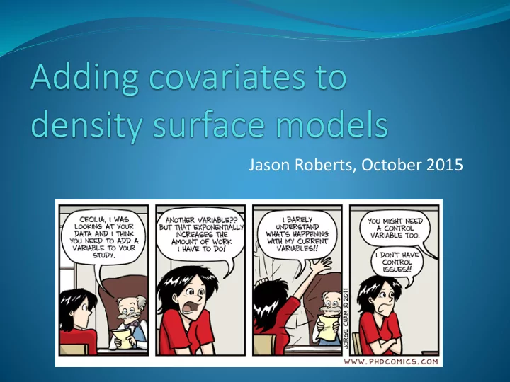
Jason Roberts, October 2015 Topics for this session Why use - PowerPoint PPT Presentation
Jason Roberts, October 2015 Topics for this session Why use covariates other than x and y? What other covariates are there? Dynamic spatial covariates: how hard can it be? Covariates for our sperm whale model Man any im images s
Jason Roberts, October 2015
Topics for this session Why use covariates other than x and y? What other covariates are there? Dynamic spatial covariates: how hard can it be? Covariates for our sperm whale model Man any im images s in in th this is presentation ar are use sed with ithout attribution. Ple lease ac accept my ap apologies an and bela lated th thanks if if I I have use sed your im image with ithout permis ission.
Why use covariates other than x and y? Three common motivations: 1. Desire for ecologically relevant covariates Tie model to ecological theory (but correlation ≠ causation!) Proximal variables better correlations better models
Indirect variables Distal variables Direct and Resource Proximal variables variables Guisan and Zimmerman (2000)
Habitat-based density models for the U.S. Atlantic and Gulf of Mexico Photo: Whit Welles
Bryde’s whales sighted on NOAA surveys in the Gulf of Mexico, 1994-2009
abundanc abundance ~ s( e ~ s(x,y x,y, , bs bs=" ="ts ts", k=60) + offset(log(area_km2)) )) edf Ref.df edf F p F p-value value s( s(x,y x,y) 10.09 59 0.368 0.00957 ** R-sq.( sq.(adj) = 0.012 Deviance explained = 49% -REML = 165.54 Scale est. = 13.017 n = 13163 13163
vs. 0.28 abundanc abundance ~ s( e ~ s(x,y x,y, , bs bs=" ="ts ts", k=60) + s(log10(Depth), bs bs=" ="ts ts", k=5) + offset(log(area_km2)) )) vs. 10.09 edf Ref.df edf Ref.df F p F p-value value s( s(x,y x,y) 1.736 44 0.203 0.00615 ** s(log10( s(log10(Depth) Depth)) 1.907 ) 1.907 4 4 2.099 0 2.099 0.01087 .01087 * * vs. 165.54 vs. 49% R-sq.( sq.(adj) = 0.0103 Deviance explained = 50.4% -RE REML ML = = 14 147. 7.78 S 78 Sca cale le es est. t. = 12 = 12.3 .394 94 n n = 13 = 1316 163
Can you interpret the term plots? Should you? Classic unimodal response What does this mean? from niche theory Plots: Read et al. (2014)
How do you interpret the effects of each term in large additive models? ? Plots: Becker et al. (2014)
Why use covariates other than x and y? Three common motivations: 1. Desire for ecologically relevant covariates Tie model to ecological theory (but correlation ≠ causation!) Proximal variables better correlations better models 2. Desire to model temporal dynamics E.g. migratory animals, especially in the ocean
Becker et al. (2014) Predicting seasonal density patterns of California cetaceans based on habitat models. Endang Species Res 23: 1-22. Summer shipboard surveys Winter aerial surveys 1991, 1993, 1996, 2001, 2005, 2008
Becker et al. (2014) Predicting seasonal density patterns of California cetaceans based on habitat models. Endang Species Res 23: 1-22.
Roberts et al. (in prep) Habitat-based density models for the U.S. Atlantic and Gulf of Mexico.
Why use covariates other than x and y? Three common motivations: 1. Desire for ecologically relevant covariates Tie model to ecological theory (but correlation ≠ causation!) Proximal variables better correlations better models 2. Desire to model temporal dynamics E.g. migratory animals, especially in the ocean 3. Need to extrapolate beyond the surveyed area Managers ask you to do this
Mannocci et al. (2014) Extrapolating cetacean densities beyond surveyed regions: habitat-based predictions in the circumtropical belt. J. Biogeogr. 42: 1267-1280.
Mannocci et al. (2014) Extrapolating cetacean densities beyond surveyed regions: habitat-based predictions in the circumtropical belt. J. Biogeogr. 42: 1267-1280. Term plots for the Globicephalinae guild model
Mannocci et al. (2014) Extrapolating cetacean densities beyond surveyed regions: habitat-based predictions in the circumtropical belt. J. Biogeogr. 42: 1267-1280. Globicephalinae density extrapolated to cells for which all covariates were within their sampled ranges.
What covariates can you use? Commonly used: Time Temporally-varying covariates Spatially-varying covariates, a.k.a. static spatial covariates Spatiotemporally-varying covariates, a.k.a. dynamic spatial covariates Not so common (discuss in later sessions, if interested): 2D smooths of environmental covariates (“interactions”) 3D smooth of x, y, time
Time, the usual ways Inter-annual effect Intra-annual effect For year round data, consider a cubic cyclic spline Wood (2006)
What about? What’s better: month (1 to 12) or day of year (1 to 365)? Probably day of year. Why discard information? What’s better: year as an integer (e.g. 2002) or a higher resolution representation of time (e.g. previous slide)? Probably the higher resolution representation Should I use time of day as a covariate? Probably not in a density surface model. Generally we are trying to estimate abundance of a population, which we do not expect to vary diurnally.
Temporally-varying covariates Not common in marine models, in my experience El Niño La Niña La Niña El Niño Howell EA, Kobayashi DR (2014) El Niño effects in the Palmyra Atoll region: oceanographic changes and bigeye tuna ( Thunnus obesus ) catch rate variability. Fish. Oceanogr. 15(6): 477-489.
Spatially-varying covariates Static maps of something, e.g.: Elevation, bathymetry, and derivatives: slope, aspect, etc. Cover type, soil type, seafloor type, and other classifications Cumulative climatologies of dynamic processes, e.g. mean annual rainfall, mean primary production Generally easy to work with: exact values for your segments from a single image, fit your model, predict over that image
Spatial resolution can be a problem Bathymetry (1/120°) Total kinetic energy (1/4°) Dissolved oxygen (1°) BAD: survey extent spans GOOD: survey extent spans POOR: survey extent spans one pixel. Can this many pixels. only four pixels. covariate provide much useful information?
What if covariates have different spatial resolutions? A common problem in gridded marine data: Regional bathymetry and derivatives (e.g. slope): 5-90 m Global bathymetry and derivatives: 1-2 km Popular remotely sensed sea surface temperature, ocean color, and primary productivity products: 4-9 km Sea ice products: generally 6.25-25 km Sea surface winds: 12.5-25 km Sea surface height and derivatives (e.g. currents): 25 km Salinity, chemistry, zooplankton, climate models: 1-5°
Resolution mismatch shows up twice 1. When you are sampling (a.k.a. interpolating) values of the covariates at your points 2. At prediction time, when it is necessary to obtain values of all covariates on grids that have the same extent, coordinate system, and cell size (and thus rows and columns) This requires you to reproject the covariate images to your common “template” grid you’ll use for predictions It may be desirable to have the cell size of this grid roughly match the effective area of your survey segments
Common approaches to this problem 1. Rescale all of your covariates to the lowest resolution covariate (e.g. using a focal or block statistic in ArcGIS) 2. Leave them at original resolutions, and then: Sample / project them with the nearest neighbor interpolator a. Sample / project them with another interpolator, such as b. linear or cubic spline
The usual suspects Nearest Neighbor Linear Cubic Spline 1 Dimension 2 Dimensions
Spatiotemporally-varying covariates Typically distributed as a time series of images Used very commonly in marine models Can be very complicated… let’s look at some of the issues...
(Hint: the forecast is mostly cloudy…) Dynamic spatial covariates: how hard can it be?
In the beginning, you saw this: Polovina et al. 2004 and this: and thought: Wow!
Basic idea of remote sensing
Basic idea of remote sensing
There are many sources of radiation h. Reflected Emissions from the Satellite (e.g. LASER, RADAR) h
Passive and active sources
Radiation comes in many wavelengths
The atmosphere absorbs radiation Clouds: a major problem for many sensors!
Level of absorption depends on wavelength
Sensors are designed to exploit this Passive sensors RADAR
Example: Landsat-TM: 7 wavelengths
These are called bands
Digital image for each band One band
Environmental variables estimated by equations that combine bands
You found NASA PO.DAAC on Google and clicked on Sea Surface Temperature…
What “level” of data do you want? Level Description 0 Real time data feed from ground control station. 1 Files of calibrated, geolocated, at-aperture radiance values for swath segments, with quality flags and error estimates. 2 Files of geophysical values (e.g. SST) for swath segments, calculated from the Level 1 data by applying an algorithm to Highest resolution – why not try it? the radiance values. 3 Files of uniform grids of geophysical values, for various spatial and temporal scales, produced by accumulating and projecting Level 2 data. 4 Same as Level 3, but with missing data filled in via interpolation, modeling, integration of data from multiple sensors, or other means.
Recommend
More recommend
Explore More Topics
Stay informed with curated content and fresh updates.
