Iterative Methods for Image Reconstruction Jeffrey A. Fessler EECS - PowerPoint PPT Presentation
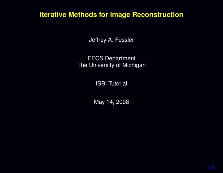
Iterative Methods for Image Reconstruction Jeffrey A. Fessler EECS Department The University of Michigan ISBI Tutorial May 14, 2008 0.0 Image Reconstruction Methods (Simplified View) Analytical Iterative (FBP) (OSEM?) (MR: iFFT) (MR:
Basis Function Considerations Mathematical • Represent f ( � r ) “well” with moderate n p (approximation accuracy) • e.g. , represent a constant (uniform) function • Orthogonality? (not essential) • Linear independence (ensures uniqueness of expansion) • Insensitivity to shift of basis-function grid (approximate shift invariance) • Rotation invariance Computational • “Easy” to compute a ij values and/or A A x Ax x • If stored, the system matrix A A A should be sparse (mostly zeros). • Easy to represent nonnegative functions e.g. , if x j ≥ 0 , then f ( � r ) ≥ 0 . A sufficient condition is b j ( � r ) ≥ 0 . 2.4
Nonlinear Object Parameterizations Estimation of intensity and shape ( e.g. , location, radius, etc.) Surface-based (homogeneous) models • Circles / spheres • Ellipses / ellipsoids • Superquadrics • Polygons • Bi-quadratic triangular Bezier patches, ... Other models θ r ) = ∑ j x j b j ( r , θ θ ) • Generalized series f ( � � • Deformable templates f ( � r ) = b ( T θ θ ( � r )) θ • ... Considerations • Can be considerably more parsimonious • If correct, yield greatly reduced estimation error • Particularly compelling in limited-data problems • Often oversimplified (all models are wrong but...) • Nonlinear dependence on location induces non-convex cost functions, complicating optimization 2.5
Example Basis Functions - 1D Continuous object 4 3.5 3 r ) 2.5 � f ( 2 1.5 1 0.5 0 2 4 6 8 10 12 14 16 18 Piecewise Constant Approximation 4 3.5 3 2.5 2 1.5 1 0.5 0 0 2 4 6 8 10 12 14 16 18 Quadratic B−Spline Approximation 4 3.5 3 2.5 2 1.5 1 0.5 0 0 2 4 6 8 10 12 14 16 18 x 2.6
Pixel Basis Functions - 2D 1 1 0.9 0.9 0.8 0.8 0.7 0.7 0.6 0.6 µ 0 (x,y) 0.5 0.5 0.4 0.4 0.3 0.3 0.2 0.2 0.1 0.1 0 0 8 8 6 6 8 8 4 6 4 6 4 4 2 2 2 2 x 2 0 0 0 0 x 1 Continuous image f ( � r ) Pixel basis approximation n p ∑ j = 1 x j b j ( � r ) 2.7
Blobs in SPECT: Qualitative α =10.4 Post−filt. OSEM (3 pix. FWHM) blob−based Post−filt. OSEM (3 pix. FWHM) rotation−based 4 4 1 1 3 3 2 2 1 1 64 64 0 0 1 64 1 64 α =0 Post−filt. OSEM (3 pix. FWHM) blob−based 4 4 1 x R ˆ x B 0 ˆ 3 3 x B 1 ˆ x 2 2 1 1 64 0 0 50 100 150 200 250 1 64 mm (2D SPECT thorax phantom simulations) 2.8
Blobs in SPECT: Quantitative Standard deviation vs. bias in reconstructed phantom images 3 Per iteration, rotation−based Per iteration, blob−based α =10.4 Per iteration, blob−based α =0 2.5 Per FWHM, rotation−based Per FWHM, blob−based α =10.4 Per FWHM, blob−based α =0 FBP 2 Standard deviation (%) 1.5 1 0.5 0 10 15 20 25 30 35 Bias (%) 2.9
Discrete-Discrete Emission Reconstruction Problem Having chosen a basis and linearly parameterized the emission density... x = ( x 1 ,..., x n p ) Estimate the emission density coefficient vector x x (aka “image”) using (something like) this statistical model: � n p � ∑ y i ∼ Poisson a ij x j + r i , i = 1 ,..., n d . j = 1 • { y i } n d i = 1 : observed counts from each detector unit • A A = { a ij } : system matrix (determined by system models) A • r i values : background contributions (determined separately) Many image reconstruction problems are “find x x given y y ” where x y x ] i )+ ε i , y i = g i ([ A i = 1 ,..., n d . Ax A x 2.10
Choice 2. System Model, aka Physics Z System matrix elements: a ij = s i ( � r ) b j ( � r ) d � r • scan geometry • collimator/detector response • attenuation • scatter (object, collimator, scintillator) • duty cycle (dwell time at each angle) • detector efficiency / dead-time losses • positron range, noncollinearity, crystal penetration, ... • ... Considerations • Improving system model can improve ◦ Quantitative accuracy ◦ Spatial resolution ◦ Contrast, SNR, detectability • Computation time (and storage vs compute-on-fly) • Model uncertainties ( e.g. , calculated scatter probabilities based on noisy attenuation map) • Artifacts due to over-simplifications 2.11
“Line Length” System Model for Tomography i th ray x 1 x 2 a ij � length of intersection 2.12
“Strip Area” System Model for Tomography i th ray x 1 x j − 1 a ij � area 2.13
(Implicit) System Sensitivity Patterns n d n d ∑ ∑ a ij ≈ s ( � r j ) = s i ( � r j ) i = 1 i = 1 Line Length Strip Area 2.14
Forward- / Back-projector “Pairs” Forward projection (image domain to projection domain): n p Z ∑ y i = s i ( � r ) f ( � r ) d � r = a ij x j = [ A A x x ] i , or ¯ y y = A A x ¯ Ax y Ax x j = 1 Backprojection (projection domain to image domain): � � n p n d ∑ ′ y A y y = A A a ij y i i = 1 j = 1 The term “forward/backprojection pair” often corresponds to an implicit choice for the object basis and the system model. ′ y ′ Sometimes A A y is implemented as B y B y y for some “backprojector” B B � = A B A A By A Least-squares solutions (for example): ′ A A ] − 1 A ′ y A ] − 1 B x = [ A y � = [ B x x ˆ A A A A A y B BA A B By y y 2.15
′ Mismatched Backprojector B B � = A B A A x x x ( PWLS − CG ) x x ( PWLS − CG ) x x x ˆ x ˆ Matched Mismatched 2.16
Horizontal Profiles 1.2 1 0.8 f ( x 1 , 32 ) 0.6 Matched Mismatched 0.4 ˆ 0.2 0 −0.2 0 10 20 30 40 50 60 70 x 1 2.17
SPECT System Modeling Collimator / Detector Complications: nonuniform attenuation, depth-dependent PSF, Compton scatter 2.18
Choice 3. Statistical Models After modeling the system physics, we have a deterministic “model:” y i ≈ g i ([ A A x x ] i ) Ax for some functions g i , e.g. , g i ( l ) = l + r i for emission tomography. Statistical modeling is concerned with the “ ≈ ” aspect. Considerations • More accurate models: ◦ can lead to lower variance images, ◦ may incur additional computation, ◦ may involve additional algorithm complexity ( e.g. , proper transmission Poisson model has nonconcave log-likelihood) • Statistical model errors ( e.g. , deadtime) • Incorrect models ( e.g. , log-processed transmission data) 2.19
Statistical Model Choices for Emission Tomography • “None.” Assume y y y − r r r = A A x x . “Solve algebraically” to find x x x . Ax x � 2 • White Gaussian noise. Ordinary least squares: minimize � y y y − A A x Ax (This is the appropriate statistical model for MR.) • Non-white Gaussian noise. Weighted least squares: minimize n p n d ∑ ∑ x � 2 x ] i ) 2 , where [ A x ] i � � y y − A W = w i ( y i − [ A y A x A x A x Ax Ax Ax a ij x j W W i = 1 j = 1 ( e.g. , for Fourier rebinned (FORE) PET data) • Ordinary Poisson model (ignoring or precorrecting for background) y i ∼ Poisson { [ A x ] i } A Ax x • Poisson model y i ∼ Poisson { [ A x ] i + r i } A x Ax • Shifted Poisson model (for randoms precorrected PET) y i = y prompt − y delay ∼ Poisson { [ A A x x ] i + 2 r i }− 2 r i Ax i i 2.20
Shifted-Poisson Model for X-ray CT A model that includes both photon variability and electronic readout noise: � 0 , σ 2 � y i ∼ Poisson { ¯ y i ( µ µ µ ) } + N Shifted Poisson approximation (matches first two moments): � y i + σ 2 � � µ )+ σ 2 � + ∼ Poisson y i ( µ µ ¯ or just use WLS... Complications: • Intractability of likelihood for Poisson+Gaussian • Compound Poisson distribution due to photon-energy-dependent detector sig- nal. X-ray statistical modeling is a current research area in several groups! 2.21
Choice 4. Cost Functions Components: • Data-mismatch term • Regularization term (and regularization parameter β ) • Constraints ( e.g. , nonnegativity) Cost function: Ψ ( x x )+ β Roughness ( x x ) = DataMismatch ( y y , A x ) x y A Ax x x Reconstruct image ˆ x by minimization: x x Ψ ( x x � argmin x x x ) x ˆ x ≥ 0 x x 0 0 Actually several sub-choices to make for Choice 4 ... Distinguishes “statistical methods” from “algebraic methods” for “ y y = A x . ” y A Ax x 2.22
Why Cost Functions? (vs “procedure” e.g. , adaptive neural net with wavelet denoising) Theoretical reasons ML is based on minimizing a cost function: the negative log-likelihood • ML is asymptotically consistent • ML is asymptotically unbiased • ML is asymptotically efficient (under true statistical model...) • Estimation: Penalized-likelihood achieves uniform CR bound asymptotically • Detection: Qi and Huesman showed analytically that MAP reconstruction out- performs FBP for SKE/BKE lesion detection (T-MI, Aug. 2001) Practical reasons • Stability of estimates (if Ψ and algorithm chosen properly) • Predictability of properties (despite nonlinearities) • Empirical evidence (?) 2.23
Bayesian Framework Given a prior distribution p ( x x x ) for image vectors x x x , by Bayes’ rule: posterior: p ( x x x | y y y ) = p ( y y y | x x ) p ( x x x x ) / p ( y y y ) so log p ( x x | y y ) = log p ( y y | x x )+ log p ( x x ) − log p ( y y ) x y y x x y • − log p ( y y | x x ) corresponds to data mismatch term (negative log-likelihood) y x • − log p ( x x x ) corresponds to regularizing penalty function Maximum a posteriori (MAP) estimator : x = argmax log p ( x x | y y ) = argmax log p ( y y | x x )+ log p ( x x ) x ˆ x y y x x x x x x x x x • Has certain optimality properties (provided p ( y y y | x x x ) and p ( x x ) are correct). x • Same form as Ψ 2.24
Choice 4.1: Data-Mismatch Term Options (for emission tomography): • Negative log-likelihood of statistical model. Poisson emission case: n d ∑ − L ( x y ) = − log p ( y y | x x ) = ([ A x ] i + r i ) − y i log ([ A x ] i + r i )+ log y i ! x x ; y y y x A Ax x A Ax x i = 1 • Ordinary (unweighted) least squares: ∑ n d 1 x ] i ) 2 2 ( y i − ˆ r i − [ A A x Ax i = 1 � � • Data-weighted least squares: ∑ σ 2 σ 2 r i , σ 2 n d 1 x ] i ) 2 / ˆ 2 ( y i − ˆ r i − [ A A x i , ˆ i = max y i + ˆ , Ax i = 1 min (causes bias due to data-weighting). σ 2 • Reweighted least-squares: ˆ i = [ A x ] i + ˆ A A ˆ x x r i • Model-weighted least-squares (nonquadratic, but convex!) n d 1 ∑ x ] i ) 2 / ([ A 2 ( y i − ˆ r i − [ A A x A x ] i + ˆ x r i ) Ax Ax i = 1 • Nonquadratic cost-functions that are robust to outliers • ... Considerations • Faithfulness to statistical model vs computation • Ease of optimization (convex?, quadratic?) • Effect of statistical modeling errors 2.25
Choice 4.2: Regularization Forcing too much “data fit” gives noisy images Ill-conditioned problems: small data noise causes large image noise Solutions : • Noise-reduction methods • True regularization methods Noise-reduction methods • Modify the data ◦ Prefilter or “denoise” the sinogram measurements ◦ Extrapolate missing ( e.g. , truncated) data • Modify an algorithm derived for an ill-conditioned problem ◦ Stop algorithm before convergence ◦ Run to convergence, post-filter ◦ Toss in a filtering step every iteration or couple iterations ◦ Modify update to “dampen” high-spatial frequencies 2.26
Noise-Reduction vs True Regularization Advantages of noise-reduction methods • Simplicity (?) • Familiarity • Appear less subjective than using penalty functions or priors • Only fiddle factors are # of iterations, or amount of smoothing • Resolution/noise tradeoff usually varies with iteration (stop when image looks good - in principle) • Changing post-smoothing does not require re-iterating Advantages of true regularization methods • Stability (unique minimizer & convergence = ⇒ initialization independence) • Faster convergence • Predictability • Resolution can be made object independent • Controlled resolution ( e.g. , spatially uniform, edge preserving) • Start with reasonable image ( e.g. , FBP) = ⇒ reach solution faster. 2.27
True Regularization Methods Redefine the problem to eliminate ill-conditioning, rather than patching the data or algorithm! Options • Use bigger pixels (fewer basis functions) ◦ Visually unappealing ◦ Can only preserve edges coincident with pixel edges ◦ Results become even less invariant to translations • Method of sieves (constrain image roughness) ◦ Condition number for “pre-emission space” can be even worse ◦ Lots of iterations ◦ Commutability condition rarely holds exactly in practice ◦ Degenerates to post-filtering in some cases • Change cost function by adding a roughness penalty / prior Ψ ( x Ψ ( x x )+ β R ( x x = argmin x ) , x ) = Ł ( x x ) x x ˆ x x x x x x x ◦ Disadvantage: apparently subjective choice of penalty ◦ Apparent difficulty in choosing penalty parameter(s), e.g. , β ( cf. apodizing filter / cutoff frequency in FBP) 2.28
Penalty Function Considerations • Computation • Algorithm complexity • Uniqueness of minimizer of Ψ ( x x x ) • Resolution properties (edge preserving?) • # of adjustable parameters • Predictability of properties (resolution and noise) Choices • separable vs nonseparable • quadratic vs nonquadratic • convex vs nonconvex 2.29
Penalty Functions: Separable vs Nonseparable Separable n p x = ∑ x ) = 1 x ′ I j = 1 x 2 • Identity norm: R ( x j / 2 x x I x 2 x Ix penalizes large values of x x , but causes “squashing bias” x n p x ) = ∑ • Entropy: R ( x x j = 1 x j log x j ( x j − µ j ) 2 n p • Gaussian prior with mean µ j , variance σ 2 x ) = ∑ j : R ( x x j = 1 2 σ 2 j n p x ) = ∑ j = 1 p ( x j , µ j , σ j ) where p ( x , µ , σ ) is Gamma pdf • Gamma prior R ( x x The first two basically keep pixel values from “blowing up.” The last two encourage pixels values to be close to prior means µ j . n p ∑ General separable form: R ( x x ) = f j ( x j ) x j = 1 Slightly simpler for minimization, but these do not explicitly enforce smoothness. The simplicity advantage has been overcome in newer algorithms. 2.30
Penalty Functions: Separable vs Nonseparable Nonseparable (partially couple pixel values) to penalize roughness Example x 1 x 2 x 3 x ) = ( x 2 − x 1 ) 2 +( x 3 − x 2 ) 2 +( x 5 − x 4 ) 2 R ( x x +( x 4 − x 1 ) 2 +( x 5 − x 2 ) 2 x 4 x 5 2 2 2 3 3 1 1 3 1 2 1 2 2 2 2 R ( x x ) = 1 R ( x x ) = 6 R ( x x ) = 10 x x x Rougher images = ⇒ larger R ( x x ) values x 2.31
Roughness Penalty Functions First-order neighborhood and pairwise pixel differences: n p 1 ∑ 2 ∑ ψ ( x j − x k ) R ( x x x ) = j = 1 k ∈ N j N j � neighborhood of j th pixel ( e.g. , left, right, up, down) ψ called the potential function Finite-difference approximation to continuous roughness measure: Z � � � � � � ∂ ∂ ∂ 2 2 2 Z � � � � � � � ∇ f ( r ) � 2 d R ( f ( · )) = � � r = ∂ x f ( � r ) + ∂ y f ( � r ) + ∂ z f ( � r ) � r . d � � � � � � � � � � � � � ∂ 2 Second derivatives also useful: � ∂ x 2 f ( � r ) ≈ f ( � r j + 1 ) − 2 f ( � r j )+ f ( � r j − 1 ) � (More choices!) � � r = � r j n p ∑ ψ ( x j + 1 − 2 x j + x j − 1 )+ ··· R ( x x x ) = j = 1 2.32
Penalty Functions: General Form n p x ) = ∑ ∑ ψ k ([ C R ( x x ] k ) where [ C x ] k = x C Cx x C Cx x c k j x j j = 1 k Example : x 1 x 2 x 3 x 4 x 5 − 1 x 2 − x 1 1 0 0 0 x 1 0 − 1 1 x 3 − x 2 0 0 x 2 x = 0 0 − 1 1 = x 5 − x 4 C x 0 x 3 C Cx − 1 x 4 − x 1 0 0 1 0 x 4 0 − 1 0 x 5 − x 2 0 1 x 5 5 ∑ ψ k ([ C R ( x x ) = x ] k ) x C Cx x k = 1 = ψ 1 ( x 2 − x 1 )+ ψ 2 ( x 3 − x 2 )+ ψ 3 ( x 5 − x 4 )+ ψ 4 ( x 4 − x 1 )+ ψ 5 ( x 5 − x 2 ) 2.33
Penalty Functions: Quadratic vs Nonquadratic x ) = ∑ ψ k ([ C R ( x x C x ] k ) x Cx k Quadratic ψ k If ψ k ( t ) = t 2 / 2 , then R ( x C ′ C x ′ C x ) = 1 x , a quadratic form. x x C C x 2 x Cx • Simpler optimization • Global smoothing Nonquadratic ψ k • Edge preserving • More complicated optimization. (This is essentially solved in convex case.) • Unusual noise properties • Analysis/prediction of resolution and noise properties is difficult • More adjustable parameters ( e.g. , δ ) � | t | ≤ δ t 2 / 2 , Example: Huber function. ψ ( t ) � δ | t |− δ 2 / 2 , | t | > δ Example: Hyperbola function. ψ ( t ) � δ 2 �� � 1 +( t / δ ) 2 − 1 2.34
Quadratic vs Non−quadratic Potential Functions 3 Parabola (quadratic) 2.5 Huber, δ =1 Hyperbola, δ =1 2 ψ ( t ) 1.5 1 0.5 0 −2 −1 0 1 2 t Lower cost for large differences = ⇒ edge preservation 2.35
Edge-Preserving Reconstruction Example Phantom Quadratic Penalty Huber Penalty 2.36
More “Edge Preserving” Regularization Chlewicki et al. , PMB, Oct. 2004: “Noise reduction and convergence of Bayesian algorithms with blobs based on the Huber function and median root prior” 2.37
Piecewise Constant “Cartoon” Objects ∠ x true 400 k−space samples |x| true 2 0.5 1 1 2 0 −2 28 28 0 −0.5 1 32 1 32 |x| "conj phase" |x| pcg quad |x| pcg edge −2 0 2 2 2 2 1 1 1 28 28 28 0 0 0 ∠ x "conj phase" ∠ x pcg quad ∠ x pcg edge 1 32 1 32 1 32 0.5 0.5 0.5 1 1 1 28 28 28 −0.5 −0.5 −0.5 1 32 1 32 1 32 2.38
Total Variation Regularization Non-quadratic roughness penalty: r ≈ ∑ Z � ∇ f ( � r ) � d � | [ C x ] k | C x Cx k Uses magnitude instead of squared magnitude of gradient. Problem: |·| is not differentiable. �� � | t | ≈ δ 1 +( t / δ ) 2 − 1 Practical solution: (hyperbola!) Potential functions 5 Total Variation 4 Hyperbola, δ =0.2 Hyperbola, δ =1 3 ψ ( t ) 2 1 0 −5 0 5 t 2.39
Total Variation Example todo: example showing blocky reconstruction with TV 2.40
Compressed Sensing aka compressive sampling or sparsity regularization θ x in terms of coefficients θ θ : Idea: find a basis B B B for representing x x θ B θ θ , where only a “small number” of θ j values are nonzero . x = B x B x Previous cost function: Ψ ( x x )+ β Roughness ( x x ) = DataMismatch ( y y , A x ) x y A Ax x x New cost function with sparsity regularization: θ θ θ Ψ ( θ θ ) = DataMismatch ( y B θ θ )+ β � θ θ � 0 y , A y AB A B � ∑ j | θ j | p � 1 / p θ � θ θ � p � θ θ � θ θ � ∞ � lim p → ∞ � θ θ � p = max j | θ j | Recall: � θ θ θ � 0 � lim p → 0 � θ θ θ � p p = ∑ j 1 { θ j � = 0 } (not a norm in the Banach sense) θ θ Because � θ θ � 0 is nonconvex, it usually is replaced with � θ θ � 1 . θ Because � θ θ � 1 is nondifferentiable, the corner is often rounded (hyperbola). � � θ B is the Harr wavelet basis, then � θ θ � 1 = B − 1 x If B 1 is similar to TV regularization. B � B B x x � For certain types of under-sampled measurements A A , “good” reconstructions are A possible! Example: radial k-space sampling for Shepp-Logan. 2.41
Penalty Functions: Convex vs Nonconvex Convex • Easier to optimize • Guaranteed unique minimizer of Ψ (for convex negative log-likelihood) Nonconvex • Greater degree of edge preservation • Nice images for piecewise-constant phantoms! • Even more unusual noise properties • Multiple extrema • More complicated optimization (simulated / deterministic annealing) • Estimator ˆ x x becomes a discontinuous function of data Y Y x Y Nonconvex examples • “broken parabola” ψ ( t ) = min ( t 2 , t 2 max ) • true median root prior: n p x )) 2 ( x j − median j ( x x ∑ R ( x x ) = where median j ( x x ) is local median x x median j ( x x ) x j = 1 Exception: orthonormal wavelet threshold denoising via nonconvex potentials! 2.42
Potential Functions 2 Parabola (quadratic) Huber (convex) Broken parabola (non−convex) 1.5 Potential Function ψ (t) 1 0.5 δ =1 0 −2 −1 0 1 2 t = x j − x k 2.43
Local Extrema and Discontinuous Estimators Ψ ( x x x ) x x x x ˆ x x Small change in data = ⇒ large change in minimizer ˆ x x . x Using convex penalty functions obviates this problem. 2.44
Augmented Regularization Functions b )+ α R ( b Replace roughness penalty R ( x x x ) with R ( x x x | b b b b ) , where the elements of b b (often binary) indicate boundary locations. b • Line-site methods • Level-set methods Joint estimation problem: Ψ ( x Ψ ( x y )+ β R ( x b )+ α R ( b x , ˆ ( ˆ b ) = argmin x , b b ) , x , b b ) = Ł ( x x | b b ) . x x b b x b x b x x ; y y x b b x , b x b x b Example: b jk indicates the presence of edge between pixels j and k : n p ( 1 − b jk ) 1 ∑ j = 1 ∑ 2 ( x j − x k ) 2 R ( x x | b b ) = x b k ∈ N j Penalty to discourage too many edges ( e.g. ): b ) = ∑ R ( b b jk . b jk • Can encourage local edge continuity • May require annealing methods for minimization 2.45
Modified Penalty Functions n p 1 ∑ 2 ∑ w jk ψ ( x j − x k ) R ( x x ) = x j = 1 k ∈ N j Adjust weights { w jk } to • Control resolution properties • Incorporate anatomical side information (MR/CT) (avoid smoothing across anatomical boundaries) Recommendations • Emission tomography: ◦ Begin with quadratic (nonseparable) penalty functions ◦ Consider modified penalty for resolution control and choice of β ◦ Use modest regularization and post-filter more if desired • Transmission tomography (attenuation maps), X-ray CT ◦ consider convex nonquadratic ( e.g. , Huber) penalty functions ◦ choose δ based on attenuation map units (water, bone, etc.) ◦ choice of regularization parameter β remains nontrivial, learn appropriate values by experience for given study type 2.46
Choice 4.3: Constraints • Nonnegativity • Known support • Count preserving • Upper bounds on values e.g. , maximum µ of attenuation map in transmission case Considerations • Algorithm complexity • Computation • Convergence rate • Bias (in low-count regions) • . . . 2.47
Open Problems • Performance prediction for nonquadratic regularization • Effect of nonquadratic regularization on detection tasks • Choice of regularization parameters for nonquadratic regularization 2.48
Summary • 1. Object parameterization: function f ( � r ) vs vector x x x • 2. System physical model: s i ( � r ) • 3. Measurement statistical model Y i ∼ ? • 4. Cost function: data-mismatch / regularization / constraints Reconstruction Method � Cost Function + Algorithm Naming convention: “criterion”-“algorithm”: • ML-EM, MAP-OSL, PL-SAGE, PWLS+SOR, PWLS-CG, . . . 2.49
Part 3. Algorithms Method = Cost Function + Algorithm Outline • Ideal algorithm • Classical general-purpose algorithms • Considerations: ◦ nonnegativity ◦ parallelization ◦ convergence rate ◦ monotonicity • Algorithms tailored to cost functions for imaging ◦ Optimization transfer ◦ EM-type methods ◦ Poisson emission problem ◦ Poisson transmission problem • Ordered-subsets / block-iterative algorithms ◦ Recent convergent versions (relaxation, incrementalism) 3.1
Why iterative algorithms? • For nonquadratic Ψ , no closed-form solution for minimizer. • For quadratic Ψ with nonnegativity constraints, no closed-form solution. • For quadratic Ψ without constraints, closed-form solutions: x � 2 x ′ R ′ W R ] − 1 A ′ W x = argmin � y y − A W 1 / 2 + x x = [ A A + R PWLS: x ˆ y A x x R x A W A R A W y x Ax Rx A WA A Wy y W W x x x x � 2 = [ A ′ A A ] − 1 A ′ y OLS: x = argmin � y y − A x x ˆ y Ax A x A A A A A y y x x x Impractical (memory and computation) for realistic problem sizes. ′ A A is sparse, but A A is not. A A A A A All algorithms are imperfect. No single best solution. 3.2
General Iteration Projection Calibration ... Measurements System Model x ( n + 1 ) x ( n ) Iteration x x x x Ψ Parameters x ( n + 1 ) = M ( x x ( n ) ) Deterministic iterative mapping: x x x 3.3
Ideal Algorithm x ⋆ � argmin Ψ ( x x x x ) (global minimizer) x x ≥ 0 x x 0 0 Properties x ⋆ if run indefinitely x ( n ) } converges to x stable and convergent { x x x x ⋆ in just a few iterations x ( n ) } gets “close” to x converges quickly { x x x x ( n ) independent of starting image x x ( 0 ) globally convergent x x lim n x fast requires minimal computation per iteration robust insensitive to finite numerical precision user friendly nothing to adjust ( e.g. , acceleration factors) parallelizable (when necessary) simple easy to program and debug flexible accommodates any type of system model (matrix stored by row or column, or factored, or projector/backprojector) Choices: forgo one or more of the above 3.4
Classic Algorithms Non-gradient based • Exhaustive search • Nelder-Mead simplex (amoeba) Converge very slowly, but work with nondifferentiable cost functions. Gradient based • Gradient descent x ( n + 1 ) � x x ( n ) − α∇Ψ � x ( n ) � x x x x x Choosing α to ensure convergence is nontrivial. • Steepest descent x ( n + 1 ) � x x ( n ) − α n ∇Ψ � x ( n ) � � x ( n ) − α∇Ψ � x ( n ) �� where α n � argmin Ψ x x x x x x x x x α Computing stepsize α n can be expensive or inconvenient. Limitations • Converge slowly. • Do not easily accommodate nonnegativity constraint. 3.5
Gradients & Nonnegativity - A Mixed Blessing Unconstrained optimization of differentiable cost functions: ∇Ψ ( x x ⋆ x x ) = 0 0 0 when x x x = x x • A necessary condition always. • A sufficient condition for strictly convex cost functions. • Iterations search for zero of gradient. Nonnegativity-constrained minimization : Karush-Kuhn-Tucker conditions � = 0 , x ⋆ � ∂ j > 0 � Ψ ( x x x ) is � ∂ x j ≥ 0 , x ⋆ j = 0 � x ⋆ x x x = x x • A necessary condition always. • A sufficient condition for strictly convex cost functions. • Iterations search for ??? ∂ ∂ x j Ψ ( x • 0 = x ⋆ x ⋆ ) is a necessary condition, but never sufficient condition. x j 3.6
Karush-Kuhn-Tucker Illustrated 6 5 4 x ) x Ψ ( x 3 2 1 Inactive constraint Active constraint 0 −4 −3 −2 −1 0 1 2 3 4 5 6 x x x 3.7
Why Not Clip Negatives? WLS with Clipped Newton−Raphson 3 Nonnegative 2 Orthant 1 0 x 2 −1 −2 −3 −6 −4 −2 0 2 4 6 x 1 Newton-Raphson with negatives set to zero each iteration. Fixed-point of iteration is not the constrained minimizer! 3.8
Newton-Raphson Algorithm x ( n + 1 ) = x x ( n ) − [ ∇ 2 Ψ � x ( n ) � � x ( n ) � ] − 1 ∇Ψ x x x x x x x Advantage : • Super-linear convergence rate (if convergent) Disadvantages : • Requires twice-differentiable Ψ • Not guaranteed to converge • Not guaranteed to monotonically decrease Ψ • Does not enforce nonnegativity constraint • Computing Hessian ∇ 2 Ψ often expensive • Impractical for image recovery due to matrix inverse General purpose remedy: bound-constrained Quasi-Newton algorithms 3.9
Newton’s Quadratic Approximation 2nd-order Taylor series: x ( n ) ) T ∇ 2 Ψ x ( n ) )+ 1 � x ( n ) � � x ( n ) � � x ( n ) � Ψ ( x x ) ≈ φ ( x x ( n ) ) � Ψ + ∇Ψ x ( n ) ) ( x x − x 2 ( x x − x ( x x − x x x ; x x x x x x x x x x x x x x x x ( n + 1 ) to the (“easily” found) minimizer of this quadratic approximation: Set x x x ( n + 1 ) � argmin φ ( x x ( n ) ) x x x x ; x x x x x x ( n ) − [ ∇ 2 Ψ � x ( n ) � � x ( n ) � ] − 1 ∇Ψ = x x x x x x Can be nonmonotone for Poisson emission tomography log-likelihood, even for a single pixel and single ray: Ψ ( x ) = ( x + r ) − y log ( x + r ) . 3.10
Nonmonotonicity of Newton-Raphson 1 0.5 0 Ψ ( x ) new −0.5 −1 old −1.5 − Log−Likelihood Newton Parabola −2 0 1 2 3 4 5 6 7 8 9 10 x 3.11
Consideration: Monotonicity An algorithm is monotonic if � x ( n + 1 ) � � x ( n ) � Ψ ≤ Ψ x ( n ) . x x , ∀ x x x x Three categories of algorithms: • Nonmonotonic (or unknown) • Forced monotonic ( e.g. , by line search) • Intrinsically monotonic (by design, simplest to implement) Forced monotonicity Most nonmonotonic algorithms can be converted to forced monotonic algorithms by adding a line-search step: x temp � M ( x x temp − x x ( n ) ) , x ( n ) d = x x x x d d x x x ( n + 1 ) � x d ( n ) where α n � argmin x ( n ) − α n d � x ( n ) − α d d ( n ) � Ψ x x d x d x x α Inconvenient, sometimes expensive, nonnegativity problematic. 3.12
Conjugate Gradient (CG) Algorithm Advantages : • Fast converging (if suitably preconditioned) (in unconstrained case) • Monotonic (forced by line search in nonquadratic case) • Global convergence (unconstrained case) • Flexible use of system matrix A A and tricks A • Easy to implement in unconstrained quadratic case • Highly parallelizable Disadvantages : • Nonnegativity constraint awkward (slows convergence?) • Line-search somewhat awkward in nonquadratic cases • Possible need to “restart” after many iterations Highly recommended for unconstrained quadratic problems ( e.g. , PWLS without nonnegativity). Useful (but perhaps not ideal) for Poisson case too. 3.13
Consideration: Parallelization Simultaneous (fully parallelizable) update all pixels simultaneously using all data EM, Conjugate gradient, ISRA, OSL, SIRT, MART, ... Block iterative (ordered subsets) update (nearly) all pixels using one subset of the data at a time OSEM, RBBI, ... Row action update many pixels using a single ray at a time ART, RAMLA Pixel grouped (multiple column action) update some (but not all) pixels simultaneously a time, using all data Grouped coordinate descent, multi-pixel SAGE (Perhaps the most nontrivial to implement) Sequential (column action) update one pixel at a time, using all (relevant) data Coordinate descent, SAGE 3.14
Coordinate Descent Algorithm aka Gauss-Siedel, successive over-relaxation (SOR), iterated conditional modes (ICM) Update one pixel at a time, holding others fixed to their most recent values: � � Ψ x new x new ,..., x new j − 1 , x j , x old j + 1 ,..., x old = argmin , j = 1 ,..., n p j 1 n p x j ≥ 0 Advantages : • Intrinsically monotonic • Fast converging (from good initial image) • Global convergence • Nonnegativity constraint trivial Disadvantages : • Requires column access of system matrix A A A • Cannot exploit some “tricks” for A A , e.g. , factorizations A • Expensive “arg min” for nonquadratic problems • Poorly parallelizable 3.15
Constrained Coordinate Descent Illustrated Clipped Coordinate−Descent Algorithm 2 1.5 1 0.5 1.5 1 2 0.5 x 2 0 −0.5 −1 0 −1.5 −2 −2 −1.5 −1 −0.5 0 0.5 1 x 1 3.16
Coordinate Descent - Unconstrained Unconstrained Coordinate−Descent Algorithm 2 1.5 1 0.5 x 2 0 −0.5 −1 −1.5 −2 −2 −1.5 −1 −0.5 0 0.5 1 x 1 3.17
Coordinate-Descent Algorithm Summary Recommended when all of the following apply: • quadratic or nearly-quadratic convex cost function • nonnegativity constraint desired • precomputed and stored system matrix A A A with column access • parallelization not needed (standard workstation) Cautions: • Good initialization ( e.g. , properly scaled FBP) essential. (Uniform image or zero image cause slow initial convergence.) • Must be programmed carefully to be efficient. (Standard Gauss-Siedel implementation is suboptimal.) • Updates high-frequencies fastest = ⇒ poorly suited to unregularized case Used daily in UM clinic for 2D SPECT / PWLS / nonuniform attenuation Under investigation for 3D helical CT reconstruction by Thibault et al. 3.18
Summary of General-Purpose Algorithms Gradient-based • Fully parallelizable • Inconvenient line-searches for nonquadratic cost functions • Fast converging in unconstrained case • Nonnegativity constraint inconvenient Coordinate-descent • Very fast converging • Nonnegativity constraint trivial • Poorly parallelizable • Requires precomputed/stored system matrix CD is well-suited to moderate-sized 2D problem ( e.g. , 2D PET), but challenging for large 2D problems (X-ray CT) and fully 3D problems Neither is ideal. . .. need special-purpose algorithms for image reconstruction! 3.19
Data-Mismatch Functions Revisited For fast converging, intrinsically monotone algorithms, consider the form of Ψ . WLS : n d n d 1 where h i ( l ) � 1 ∑ ∑ x ] i ) 2 = 2 w i ( y i − l ) 2 . Ł ( x x x ) = 2 w i ( y i − [ A A x h i ([ A A x x ] i ) , Ax Ax i = 1 i = 1 Emission Poisson (negative) log-likelihood : n d n d ∑ ∑ Ł ( x x ) = ([ A x ] i + r i ) − y i log ([ A x ] i + r i ) = h i ([ A x ] i ) x A Ax x A Ax x A Ax x i = 1 i = 1 where h i ( l ) � ( l + r i ) − y i log ( l + r i ) . Transmission Poisson log-likelihood : n d n d � � � � ∑ ∑ x ] i + r i x ] i + r i b i e − [ A A x b i e − [ A A x Ax Ax Ł ( x x x ) = − y i log = h i ([ A A x x ] i ) Ax i = 1 i = 1 where h i ( l ) � ( b i e − l + r i ) − y i log � b i e − l + r i � . MRI, polyenergetic X-ray CT, confocal microscopy, image restoration, ... All have same partially separable form. 3.20
General Imaging Cost Function General form for data-mismatch function: n d ∑ Ł ( x x ) = h i ([ A x ] i ) x A Ax x i = 1 General form for regularizing penalty function: x ) = ∑ ψ k ([ C R ( x x ] k ) x C x Cx k General form for cost function: n d ∑ x ] i )+ β ∑ Ψ ( x x )+ β R ( x ψ k ([ C x ) = Ł ( x x ) = h i ([ A x ] k ) x x x A Ax x Cx C x i = 1 k Properties of Ψ we can exploit: • summation form (due to independence of measurements) • convexity of h i functions (usually) • summation argument (inner product of x x with i th row of A A ) x A Most methods that use these properties are forms of optimization transfer . 3.21
Optimization Transfer Illustrated x ) x x ) and φ ( n ) ( x x Ψ ( x Surrogate function Cost function x ( n ) x x ( n + 1 ) x x x 3.22
Optimization Transfer General iteration: x ( n + 1 ) = argmin � x ( n ) � φ x x x x x x ; x x ≥ 0 x x 0 0 Monotonicity conditions (cost function Ψ decreases provided these hold): • φ ( x x ( n ) ) = Ψ ( x x ( n ) ; x x ( n ) ) x x x (matched current value) � � • ∇ x x φ ( x x ( n ) = ∇Ψ ( x � � x ( n ) ) x x x x ) (matched gradient) x ; x x � � x ( n ) x x = x x x = x x x x x • φ ( x x ( n ) ) ≥ Ψ ( x x ) ∀ x x ≥ 0 x x x x 0 (lies above) x ; x 0 These 3 (sufficient) conditions are satisfied by the Q function of the EM algorithm (and its relatives like SAGE). The 3rd condition is not satisfied by the Newton-Raphson quadratic approxima- tion, which leads to its nonmonotonicity. 3.23
Optimization Transfer in 2d 3.24
Optimization Transfer cf EM Algorithm E-step: choose surrogate function φ ( x x ( n ) ) x x x ; x M-step: minimize surrogate function x ( n + 1 ) = argmin � x ( n ) � φ x x x x x x ; x x x ≥ 0 0 x 0 Designing surrogate functions • Easy to “compute” • Easy to minimize • Fast convergence rate Often mutually incompatible goals . .. compromises 3.25
Convergence Rate: Slow High Curvature Small Steps Slow Convergence φ Φ x Old New 3.26
Convergence Rate: Fast Low Curvature Large Steps Fast Convergence φ Φ x Old New 3.27
Tool: Convexity Inequality g ( x ) x α x 1 +( 1 − α ) x 2 x 1 x 2 ⇒ g ( α x 1 +( 1 − α ) x 2 ) ≤ α g ( x 1 )+( 1 − α ) g ( x 2 ) for α ∈ [ 0 , 1 ] g convex = More generally: α k ≥ 0 and ∑ k α k = 1 = ⇒ g ( ∑ k α k x k ) ≤ ∑ k α k g ( x k ) . Sum outside! 3.28
Example 1: Classical ML-EM Algorithm Negative Poisson log-likelihood cost function (unregularized): n d ∑ Ψ ( x x ) = h i ([ A x ] i ) , h i ( l ) = ( l + r i ) − y i log ( l + r i ) . x A x Ax i = 1 Intractable to minimize directly due to summation within logarithm. ( n ) x ( n ) ] i + r i ): = [ A Clever trick due to De Pierro (let ¯ A x y Ax i � �� � ( n ) n p n p a ij x x j ∑ ∑ j ( n ) [ A x ] i = a ij x j = . A x ¯ Ax y i ( n ) ( n ) y ¯ x j = 1 j = 1 i j Since the h i ’s are convex in Poisson emission model: � n p � �� �� � � � � ( n ) ( n ) n p a ij x a ij x x j x j ∑ ∑ j j ( n ) ( n ) h i ([ A x ] i ) = h i ≤ A x ¯ h i ¯ Ax y y i i ( n ) ( n ) ( n ) ( n ) y ¯ x y ¯ x j = 1 j = 1 i j i j � � � � ( n ) n p n d n d a ij x x j ∑ ∑ ∑ � x ( n ) � Ψ ( x x ] i ) ≤ φ j ( n ) � x ) = h i ([ A x A Ax x x x x ; x x h i y ¯ i ( n ) ( n ) y ¯ x i = 1 i = 1 j = 1 i j Replace convex cost function Ψ ( x x ) with separable surrogate function φ ( x x ( n ) ) . x x x ; x x 3.29
“ML-EM Algorithm” M-step E-step gave separable surrogate function: � � � � ( n ) n p n d a ij x x j ∑ ∑ � x ( n ) � � x ( n ) � � x ( n ) � φ φ j , where φ j j ( n ) � x x = x x h i . x x ; x x j ; x x j ; x y ¯ i ( n ) ( n ) y ¯ x j = 1 i = 1 i j M-step separates: x ( n + 1 ) = argmin � x ( n ) � � x ( n ) � φ ( n + 1 ) φ j = ⇒ x = argmin , j = 1 ,..., n p x x x x ; x x x x j ; x x j x j ≥ 0 x x ≥ 0 0 0 x Minimizing: �� � ∂ n d n d � � � y i ∑ ∑ � x ( n ) � φ j ( n ) ( n ) a ij ˙ � x = h i i x j / x = 1 − = 0 . x j ; x y ¯ a ij ∂ x j � j ( n ) ( n ) i x j / x y ¯ � i = 1 i = 1 x j = x ( n + 1 ) j j Solving (in case r i = 0 ): � � � � n d n d y i ∑ ∑ ( n + 1 ) ( n ) = x / , j = 1 ,..., n p x a ij a ij j j x ( n ) ] i [ A A x Ax i = 1 i = 1 • Derived without any statistical considerations, unlike classical EM formulation. • Uses only convexity and algebra. • Guaranteed monotonic: surrogate function φ satisfies the 3 required proper- ties. • M-step trivial due to separable surrogate . 3.30
ML-EM is Scaled Gradient Descent � � � � n d n d y i ∑ ∑ ( n + 1 ) ( n ) = x / x a ij a ij j j ( n ) y ¯ i = 1 i = 1 i � � �� � � n d n d y i ∑ ∑ ( n ) ( n ) = x j + x − 1 / a ij a ij j ( n ) y ¯ i = 1 i = 1 i � � ( n ) ∂ x � x ( n ) � j Ψ ( n ) = x j − , j = 1 ,..., n p x x ∂ x j n d ∑ i = 1 a ij x ( n + 1 ) = x x ( n ) + D � x ( n ) � x ( n ) ) ∇Ψ D ( x x x x D x x x This particular diagonal scaling matrix remarkably • ensures monotonicity, • ensures nonnegativity. 3.31
Consideration: Separable vs Nonseparable Separable Nonseparable 2 2 1 1 0 0 x 2 x 2 −1 −1 −2 −2 −2 0 2 −2 0 2 x 1 x 1 Contour plots: loci of equal function values. Uncoupled vs coupled minimization. 3.32
Separable Surrogate Functions (Easy M-step) The preceding EM derivation structure applies to any cost function of the form n d ∑ Ψ ( x x ) = h i ([ A x ] i ) . x A x Ax i = 1 cf ISRA (for nonnegative LS), “convex algorithm” for transmission reconstruction Derivation yields a separable surrogate function n p ∑ � x ( n ) � � x ( n ) � � x ( n ) � Ψ ( x x ) ≤ φ , where φ φ j x x x x x = x x x ; x x x ; x x j ; x j = 1 M-step separates into 1D minimization problems (fully parallelizable): x ( n + 1 ) = argmin � x ( n ) � � x ( n ) � φ ( n + 1 ) φ j = ⇒ x = argmin , j = 1 ,..., n p x x x x x x x ; x x j ; x j x ≥ 0 x 0 x j ≥ 0 x 0 Why do EM / ISRA / convex-algorithm / etc. converge so slowly? 3.33
Separable vs Nonseparable Ψ Ψ φ φ Separable Nonseparable Separable surrogates ( e.g. , EM) have high curvature . .. slow convergence. Nonseparable surrogates can have lower curvature . .. faster convergence. Harder to minimize? Use paraboloids (quadratic surrogates). 3.34
Recommend
More recommend
Explore More Topics
Stay informed with curated content and fresh updates.
