? iPEPS 0 0 . 189(2) 0 . 217(4) 0 . 25 2D tensor network ansatz - PowerPoint PPT Presentation

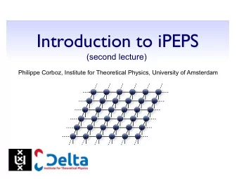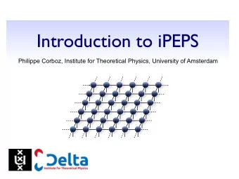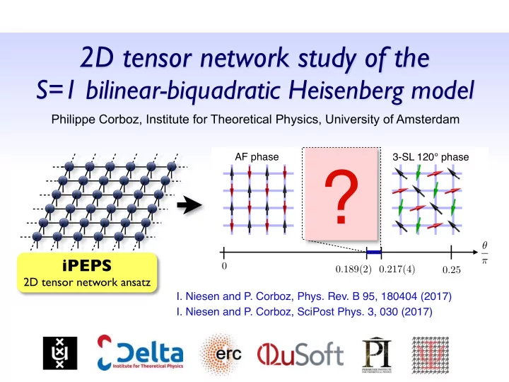
2D tensor network study of the S=1 bilinear-biquadratic Heisenberg model Philippe Corboz, Institute for Theoretical Physics, University of Amsterdam AF phase Haldane phase 3-SL 120° phase ? θ iPEPS π 0 0 . 189(2) 0 . 217(4) 0 . 25 2D tensor network ansatz I. Niesen and P. Corboz, Phys. Rev. B 95, 180404 (2017) I. Niesen and P. Corboz, SciPost Phys. 3, 030 (2017)

2D tensor network study of the S=1 bilinear-biquadratic Heisenberg model Philippe Corboz, Institute for Theoretical Physics, University of Amsterdam Ido Niesen AF phase Haldane phase 3-SL 120° phase ? θ iPEPS π 0 0 . 189(2) 0 . 217(4) 0 . 25 2D tensor network ansatz I. Niesen and P. Corboz, Phys. Rev. B 95, 180404 (2017) I. Niesen and P. Corboz, SciPost Phys. 3, 030 (2017)

Outline ‣ Motivation ✦ SU(3) Heisenberg model & spin-nematic phases & benchmark problem ‣ Method ✦ Introduction to tensor networks and iPEPS ✦ Optimization ‣ Results ✦ iPEPS results: 2 new phases ‣ Conclusion ‣ Other recent work ✦ iPEPS vs iMPS on infinite cylinders

S=1 bilinear-biquadratic Heisenberg model on a square lattice bilinear biquadratic cos( θ ) S i · S j + sin( θ ) ( S i · S j ) 2 X H = SU(2) symmetry h i,j i S=1 operators • Motivation I: SU(3) Heisenberg model ( θ = π / 4) Experiments on alkaline-earth atoms in optical lattices • Motivation II: Spin nematic phases Unusual properties of NiGa 2 S 4 / Ba 3 NiSb 2 O 9 • Motivation III: Benchmark problem for iPEPS Discover new phases?

Motivation I: SU(N) Heisenberg models S=1/2 operators X • N=2: H = S i S j Néel order h i,j i local basis states: | "i , | #i

Motivation I: SU(N) Heisenberg models P ij i j i j X • N=2: H = P ij Néel order h i,j i | o i , | o i local basis states: • N=3 Ground state?? • N=4

Nuclear spin : 87 Sr I = 9 / 2 N max = 2 I + 1 = 10 • N=3 | o i | I z = 3 / 2 i Identify nuclear | o i | I z = 1 / 2 i spin states with | o i | I z = � 1 / 2 i colors: • N=4 | o i | I z = � 3 / 2 i

Nuclear spin : 87 Sr I = 9 / 2 N max = 2 I + 1 = 10 • N=3 Cannot use QMC because of the sign problem !!! • N=4

SU(N) Heisenberg models SU(3) square/triangular: SU(3) honeycomb: Plaquette state SU(3) kagome: 3-sublattice Néel order Simplex solid state Zhao, Xu, Chen, Wei, Qin, Zhang, Xiang, PRB 85 (2012); Bauer, PC, et al., PRB 85 (2012) PC, Penc, Mila, Läuchli, PRB 86 (2012) PC, Läuchli, Penc, Mila, PRB 87 (2013) ) SU(4) square: SU(4) honeycomb: 3-color quantum Potts: Dimer-Néel order spin-orbital (4-color) liquid superfluid phases PC, Lajkó, Läuchli, Penc, Mila, PRX 2 (‘12) PC, Läuchli, Penc, Troyer, Messio, PC, Mila, PRB 88 (2013) Mila, PRL 107 (‘11)

SU(3) Heisenberg model on the square lattice X • N=3: H = P ij h i,j i | o i , | o i i , | o i local basis states: • Product state ansatz: different colors on neighboring sites ... • Infinite classical ground state degeneracy!

SU(3) Heisenberg model on the square lattice • Degeneracy lifted by quantum fluctuations: 3 sublattice Néel order • Exact diagonalization & linear flavor wave theory T. A. Tóth, A. M. Läuchli, F. Mila & K. Penc, PRL 105 (2010) • DMRG & iPEPS Bauer, PC, Läuchli, Messio, Penc, Troyer & Mila, PRB 85 (2012) Stability of 3-sublattice phase in an extended parameter space?

Stability of 3-sublattice phase away from SU(3) point? cos( θ ) S i · S j + sin( θ ) ( S i · S j ) 2 X H = h i,j i θ = π / 4 SU(3) Heisenberg model • ED + linear flavor wave theory: 3-sublattice state has finite extension Tóth, Läuchli, Mila & Penc, PRB 85 (2012) • Compatible results: series expansion Oitmaa & Hamer, PRB 87 (2013) Figure from Tóth, et al. PRB 85 (2012) ➡ Can we reproduce this with systematic iPEPS simulations?

Motivation II: Spin nematic phases • Spin nematic phase: vanishing magnetic moment: h S x i = h S y i = h S z i = 0 but still breaking SU(2) symmetry due to non-vanishing higher order moments. z Tóth, et al., PRB 85 (2012) • Example (S=1): | 0 i vanishing magnetic moment, but y NiGa 2 S 4 x h ( S z ) 2 i = 0 6 = h ( S x ) 2 i = h ( S y ) 2 i = 1 ➡ Anisotropic spin fluctuations breaking SU(2) symmetry • Possible realization: NiGa 2 S 4 Tsunetsugu & Arikawa, J. Phys. Soc. Jap. 75 (2006) Tsunetsugu & Arikawa, J. Phys. Cond. Mat. 19 (2007) Läuchli, Mila & Penc, PRL 97 (2006) Bhattacharjee, Shenoy & Senthil, PRB 74 (2006) Nakatsuji et al., Science 309 (2005)

Motivation III: benchmark problem for iPEPS • Negative sign problem controlled, systematic study has been lacking ➡ Obtain accurate estimate of the phase boundaries with iPEPS! ➡ turned out to be more complicated but also much richer than expected! • Accessible by QMC: K. Harada and N. Kawashima, J. Phys. Soc. Jpn. 70 (2001) K. Harada and N. Kawashima, PRB 65(5), 052403 (2002)

Introduction to iPEPS

Tensor network ansatz for a wave function {| "i , | #i } 2 basis states per site: Lattice: 2 6 basis states 1 2 3 4 5 6 2 6 coefficients � State: | Ψ ⇥ = Ψ i 1 i 2 i 3 i 4 i 5 i 6 | i 1 � i 2 � i 3 � i 4 � i 5 � i 6 ⇥ i 1 i 2 i 3 i 4 i 5 i 6 Tensor/multidimensional array Tensor network : matrix product state ( MPS ) d b e a c Big tensor Ψ i 1 i 2 i 3 i 4 i 5 i 6 A B C D F E bond D dimension i 1 i 2 i 3 i 4 i 5 i 6 i 1 i 2 i 3 i 4 i 5 i 6 X i 6 = ˜ Ψ i 1 i 2 i 3 i 4 i 5 i 6 A a i 1 B ab i 2 C bc i 3 D cd i 4 E de i 5 F e Ψ i 1 i 2 i 3 i 4 i 5 i 6 ≈ abcde Efficient vs poly( ,N) numbers exp(N) many numbers D representation!

“Corner” of the Hilbert space Ground states (local H) ★ GS of local H’s are less entangled than a Hilbert random state in the Hilbert space ★ Area law of the entanglement entropy space S ( L ) ∼ L d − 1 . . . . . . A L . . . . . .

MPS & PEPS 1D 2D MPS Snake MPS Matrix-product state (underlying ansatz of DMRG) Bond dimension D 1 2 3 4 5 6 7 8 L Physical indices (lattices sites) S. R. White, PRL 69, 2863 (1992) Fannes et al., CMP 144, 443 (1992) Östlund, Rommer, PRL 75, 3537 (1995) Computational cost: ∝ exp( L )

MPS & PEPS 1D 2D PEPS (TPS) MPS projected entangled-pair state Matrix-product state (tensor product state) (underlying ansatz of DMRG) Bond dimension D Bond dimension D 1 2 3 4 5 6 7 8 Physical indices (lattices sites) Verstraete and Cirac, cond-mat/0407066 Computational cost: Nishino, Hieida, Okunishi, Maeshima, Akutsu, and Gendiar, Prog. Theor. Phys. 105, 409 (2001). ∝ poly ( L, D ) Nishio, Maeshima, Gendiar, and Nishino, cond-mat/0401115

Infinite PEPS (iPEPS) 1D 2D iMPS iPEPS infinite matrix-product state infinite projected entangled-pair state A A A A A A A A A A A A A A A A A A A A A A A A A A A A A A A A A A A A Jordan, Orus, Vidal, Verstraete, Cirac, PRL (2008) ★ Work directly in the thermodynamic limit: No finite size and boundary effects!

iPEPS with arbitrary unit cells 1D 2D iMPS iPEPS infinite matrix-product state with arbitrary unit cell of tensors D A B C D A H E F G H E D B D A C A H E F G H E B D D A C A H E F G H E here: 4x2 unit cell PC, White, Vidal, Troyer, PRB 84 (2011) ★ Run simulations with different unit cell sizes ★ Systematically compare variational energies

Overview: Tensor network algorithms (ground state) MPS iPEPS TN ansatz (variational) Find the best Compute (ground) state observables | ˜ � ˜ Ψ | O | ˜ Ψ � Ψ ⇥ Contraction of the iterative optimization tensor network imaginary time of individual tensors evolution (energy minimization)

Optimization via imaginary time evolution β → ∞ • Idea: exp( � β ˆ | Ψ GS i H ) | Ψ i i τ = β /n ! n ! n Y Trotter-Suzuki exp( − β ˆ X ˆ X ˆ exp( − τ ˆ H ) = exp( − β H b ) = exp( − τ H b ) H b ) ≈ decomposition: b b b • 1D: exp( − τ ˆ H b ) ... ... • At each step: apply a two-site operator to a bond and truncate bond back to D √ √ V † U U s ˜ sV ˜ s SVD Keep D largest singular values T ime E volving B lock D ecimation (TEBD) algorithm Note: MPS needs to be in canonical form

Optimization via imaginary time evolution exp( − τ ˆ H b ) • 2D: same idea: apply to a bond and truncate bond back to D • However , SVD update is not optimal (because of loops in PEPS)! simple update (SVD) full update Jiang et al, PRL 101 (2008) Jordan et al, PRL 101 (2008) ★ “local” update like in TEBD ★ Take the full wave function into account for truncation ★ Cheap, but not optimal (e.g. overestimates magnetization ★ optimal, but computationally more in S=1/2 Heisenberg model) expensive ★ reasonable energy estimates ★ Fast-full update [Phien et al, PRB 92 (2015)]

Overview: iPEPS simulations • interacting spinless fermions ‣ honeycomb & square lattice • t-J model & Hubbard model iPEPS is a very ‣ square lattice competitive • SU(N) Heisenberg models variational method! ‣ N=3 square, triangular, kagome & honeycomb lattice ‣ N=4 square, honeycomb & checkerboard lattice ‣ N=5 square lattice Find new physics ‣ N=6 honeycomb lattice thanks to (largely) • frustrated spin systems unbiased simulations ‣ Shastry-Sutherland model ‣ Heisenberg model on kagome lattice ‣ Bilinear-biquadratic S=1 Heisenberg model ‣ Kitaev-Heisenberg model ‣ J1-J2 Heisenberg model • and many more...