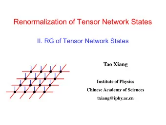
Renormalization of tensor network states Tao Xiang Institute of - PowerPoint PPT Presentation
Renormalization of tensor network states Tao Xiang Institute of Physics, Chinese Academy of Sciences Collaborators: Zhiyuan Xie, Jing Chen, Jifeng Yu, Xin Kong (IOP) Bruce Normand (Renmin University of China) Outline Issue to
Renormalization of tensor network states Tao Xiang Institute of Physics, Chinese Academy of Sciences Collaborators: Zhiyuan Xie, Jing Chen, Jifeng Yu, Xin Kong (IOP) Bruce Normand (Renmin University of China)
Outline Issue to address: How to renormalize classical or quantum statistical models accurately and efficiently 1. Brief introduction to the tensor renormalization 2. HOTRG: tensor renormalization based on the higher- order singular value decomposition 3. PESS: Projected Entangled Simplex State representation of quantum many-body wave function
Idea of Renormalization Group H 0 H 1 H 2 Energy Ernst Stueckelberg ••• ••• H eff RG iteration coarse graining : refine the wavefunction by local unitary transformations
Idea of Numerical Renormalization Group ∞ = ∑ ψ To represent a targeted state f n 0 l l = 1 l D by an approximate wavefunction using a ≈ ∑ ψ f n limited number of many-body basis states 0 l l = 1 l D = ∑ ψ ψ such that their overlap is maximized f f 0 0 l l = 1 l Key issue: How to determine these optimal basis states?
Evolution of Numerical Renormalization Group Stage I: Wilson NRG 1975 - 0 Dimensional problems (single impurity Kondo model) K. Wilson Stage II: DMRG 1992 - most accurate method for 1D quantum lattice models S R White Stage III: Renormalization of tensor network states 2D or higher dimensional quantum/classical models
What are tensor-network states/models All classical and quantum lattice models are or can be represented as tensor network models Ground state wavefunctions of quantum lattice models can be represented as tensor-network states
Example: tensor-network representation of Ising model ∑ 𝐼 = � 𝐼 ∎ H= -J S S i j ij ∎ 𝑎 = Tr exp − β 𝐼 = Tr � exp − β 𝐼 ∎ ∎ = Tr � 𝑈 𝑇 𝑗 𝑇 𝑘 𝑇 𝑙 𝑇 𝑚 { 𝑇 } 𝑇 𝑗 𝑇 𝑘 𝑇 𝑗 𝑇 𝑘 𝑇 𝑙 𝑇 𝑚 = exp − β 𝐼 ∎ = 𝑈 𝑇 𝑙 𝑇 𝑚
Quantum lattice model d-di dimens nsion onal al quant antum um model del = (d+1) 1)-di dimens nsion onal al clas assical al mode del under the framework of path integration 𝑛 Virtual basis state Physical state 𝑧 𝑦 𝑦𝑦 Many-parameter y' variational wavefunction the tensor elements are unknown and need to be determined
Questions to be solved by the tensor renormalization group Classi ssica cal sta tatisti stica cal model How to trace out all tensor indices? Quant antum um lattice e mode del 1. How to determine all local tensor elements? 2. How to trace out all tensors to obtain the expectation values?
How to renormalize tensor-network states? HOTRG: coarse graining tensor renormalization by the higher order singular value decomposition H.C. Jiang, et al, PRL 101, 090603 (2008) Z. Y. Xie et al, PRL 103, 160601 (2009) H. H. Zhao, et al, PRB 81, 174411 (2010) Z. Y. Xie et al, PRB 86, 045139 (2012)
HOTRG: Coarse graining tensor renormalization based on HOSVD Higher order singular value decompostion (HOSVD) Step 1: coarse graining To contract two local tensors into one D D 2 D x = ( x 1 , x 2 ) , x’ = ( x’ 1 , x’ 2 )
HOTRG: Coarse graining tensor renormalization based on HOSVD Step 2: determine the unitary transformation matrices By the higher order singular value decomposition
Singular value decomposition of matrix Schmidt decomposition Singular value decomposition N ∑ ∑ ψ = Λ = Λ n n f U V n sys env , , ij i n n j n n = 1 n D ∑ ≈ Λ Λ n U V 2 is the eigenvalue of reduced , , i n n j n density matrix = 1 n ψ = ∑ f i j | i 〉 sys | j 〉 env ij sys env , i j System Environment
Higher order singular value decompostion (HOSVD) Generalization of the singular value decomposition of matrixs to tensors Core tensor all-orthogonal: pseudo-diagonal / ordering: low-rank approximation for tensors L. de Latheauwer, B. de Moor, and J. Vandewalle, SIAM, J. Matrix Anal. Appl, 21, 1253 (2000).
HOTRG: Coarse graining tensor renormalization based on HOSVD Step 3: renormalize the tensor cut the tensor dimension according to the norm of the core tensor if ε 1 < ε 2 , U (n) = U L if ε 1 > ε 2 , U (n) = U R truncation error = min( ε 1 , ε 2 )
Critical Temperature of 3D Ising model Bond dimension
Critical Temperature of 3D Ising model 4.51152469(1) HOTRG D = 23 Other RG methods
Magnetization of 3D Ising model Xie et al, PRB 86,045139 (2012) HOTRG (D=14): 0.3295 Monte Carlo: 0.3262 Series Expansion: 0.3265 Relative difference is less than 10 -5 MC data: A. L. Talapov, H. W. J. Blote, J. Phys. A: Math. Gen. 29, 5727 (1996).
Specific Heat of 3D Ising model D = 14 Solid line: Monte Carlo data from X. M. Feng, and H. W. J. Blote, Phys. Rev. E 81, 031103 (2010)
2D Quantum Ising model 2D QuantumTransverse Ising Model at T = 0K
Novel Tensor-Network States Projected Entangled Simplex State (PESS) arXiv:1307.5696
Basic properties of quantum many-body wavefunction | Area Law of Entanglement Entropy Entanglement Entropy between A and B B 𝑻 𝒇𝒇𝒇 ~ 𝑶 ~ 𝐦𝐦 χ N A χ ~ 𝒇 𝑶 minimal number of basis states needed grows exponentially with system size
Basic properties of quantum many-body wavefunction What kind of wavefunctions satisfy the entanglement area law? Area Law of Entanglement Entropy Entanglement Entropy between A and B B 𝑻 𝒇𝒇𝒇 ~ 𝑶 ~ 𝐦𝐦 χ N A χ ~ 𝒇 𝑶 minimal number of basis states needed grows exponentially with system size
The Answer: tensor-network states 1 dimension Matrix product state (MPS) Multi-scale entanglement renormalization ansatz (MERA) 2 or higher dimensions Projected entangled pair state (PEPS) = tensor product state …… Projected Entangled Simplex State (PESS)
1D: Matrix product state | Matrix product state (MPS) dD 2 L parameters Ψ = ∑ ( ) m [ ]... [ ] ... Tr A m A m m m 1 1 L L α β m m 1 L A αβ [ m ] m 1 m 2 m 3 … … m L-1 m L
1D: Matrix product state Ostlund and Rommer, PRL 75 , 3537 (1995) It is the wavefunction generated by the DMRG Can be taken as an efficient trial wave function in 1D Matrix product state (MPS) Ψ = ∑ ( ) m [ ]... [ ] ... Tr A m A m m m 1 1 L L α β m m 1 L A αβ [ m ] m 1 m 2 m 3 … … m L-1 m L
Example AKLT valence bond solid state 1 1 2 ∑ A S=1 spin is a symmetric ( ) 2 = ⋅ + ⋅ + H S S S S + + 1 1 i i i i superposition of two S=1/2 spins 2 3 3 i m m α β α β = A αβ [ m ] A αβ [ m ] virtual S=1/2 spin ∑ ( ) Ψ = [ ]... [ ] ... Tr A m A m m m 1 L 1 L A αβ [ m ] : m m 1 L To project two virtual S=1/2 states, α and β , − 0 0 1 0 0 2 − = = = [ 1] [0] [1] A A A onto a S=1 state m 0 1 2 0 0 0 Affleck, Kennedy, Lieb, Tasaki, PRL 59 , 799 (1987)
Matrix Product State and Haldane Conjecture ∑ = ⋅ Integer antiferromagnetic H S S + Heisenberg spin system 1 i i has a finite excitation gap i Haldane Ni 2+ S = 1 Energy gap Y 2 BaNiO 5
AKLT valence bond solid state in 2D S = 2 Virtual basis state Physical state 𝑑 𝑏 𝑐 𝑈 𝑏𝑏𝑏𝑏 [ 𝑛 𝑗 ] = 𝑛 𝑗 d 𝐼 = � 𝑄 4 ( 𝑗 , 𝑘 ) 𝑗𝑘 To project two S=2 spins on sites i and j onto a total spin S=4 state Verstraete, Cirac 04
2D tensor network state: Projected Entangled Pair State (PEPS) Virtual basis state Physical state 𝑛 𝑧 𝑦 𝑦𝑦 𝑈 𝑦𝑦 ′ 𝑧𝑧 ′ [ 𝑛 ] = y' Verstraete, Cirac, arXiv:0407066
Projected Entangled Pair State (PEPS) Virtual basis state Physical state Successfully applied to the quantum spin models on honeycomb and square lattices But, difficult to obtain a converged result if applied to the AFM Heisenberg or other models on the Kagome or other frustrated lattices Kagome Lattice
S=1/2 Kagome Heisenberg model: Z 2 spin liquid Depenbrock,McCulloch,Schollwock, PRL 109, 067201 (2012) Ground state energy obtained with different methods
Projected Entangled Simplex States (PESS) Projection tensor Simplex tensor Virtual spins at each simplex (here triangle), instead of at each pair, form a maximally entangled state Remove the geometry frustration: The PESS wavefunction on the Kagome lattice is defined on the decorated honeycomb lattice (no frustration)
Simplex Solid States D. P. Arovas, Phys. Rev. B 77 , 104404 (2008) Example: S = 2 spin model on the Kagome lattice A S = 2 spin is a symmetric superposition of two virtual S = 1 spins Three virtual spins at each triangle form a spin singlet Projection tensor Simplex tensor
S=2 Simplex Solid State on the Kagome Lattice Local tensors Parent Hamiltonians or antisymmetric tensor 𝐵 𝑏𝑏 [ 𝜏 ] = 1 1 2 𝜏 C-G coefficients 𝑏 𝑐 P n : projection operator Projection tensor Simplex tensor
Projected Entangled Simplex State (PESS) Kagome Lattice 3-PESS form a decorated honeycomb lattice 5-PESS form a decorated square lattice
Recommend
More recommend
Explore More Topics
Stay informed with curated content and fresh updates.
