Ionospheric Models at the NOAA Space Weather Prediction Center - PowerPoint PPT Presentation
Ionospheric Models at the NOAA Space Weather Prediction Center Rodney Viereck Rashid Akmaev, David Anderson 1 , Mihail Codrescu, Tzu-Wei Fang 1 , Mariangle Fedrizzi 1 , Tim Fuller-Rowell 1 , Chih-Ting Hsu 1 , Paul Lotoaniu 1 , Naomi Maruyama 1
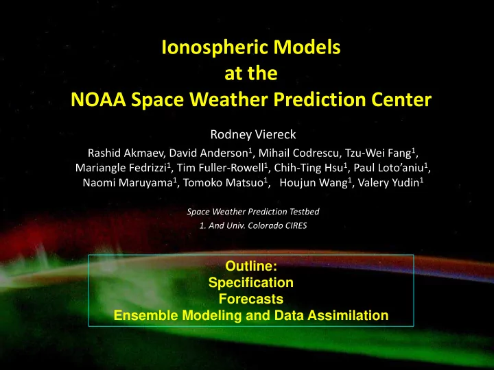
Ionospheric Models at the NOAA Space Weather Prediction Center Rodney Viereck Rashid Akmaev, David Anderson 1 , Mihail Codrescu, Tzu-Wei Fang 1 , Mariangle Fedrizzi 1 , Tim Fuller-Rowell 1 , Chih-Ting Hsu 1 , Paul Loto’aniu 1 , Naomi Maruyama 1 , Tomoko Matsuo 1 , Houjun Wang 1 , Valery Yudin 1 Space Weather Prediction Testbed 1. And Univ. Colorado CIRES Outline: Specification Forecasts Ensemble Modeling and Data Assimilation
Space Weather Prediction Center Operations – R & D – Space Weather Forecast Office Space Weather Prediction Testbed Improving Products and Services Research-to-Operations • Applied Research • Model Development • Model Test/Evaluation • Model Transition • Operations Support Operations-to-Research • Customer Requirements • Observation Requirements • Research Requirements Putting out daily forecast since 1965. Specifications; Current conditions Forecast; Conditions tomorrow Watches; Conditions are favorable for storm Warnings; Storm is imminent with high probability Alerts; observed conditions meeting or exceeding storm thresholds IES 2015 2 12 May, 2015
SWPC Models Solar • – Wang Sheeley Arge (USAF) • Heliosphere – Enlil (George Masson U.) • Magnetosphere – Space Weather Modeling Framework (U. Mich.) – OVATION Prime 2013 (JHU APL) • Ionosphere – D-RAP: D-Region Absorption Product – US-TEC: US Total Electron Content – CTIPe: Coupled Thermosphere Ionosphere Plasmasphere with electrodynamics – GIP: CTIPe ionosphere only – IPE: Ionosphere-Plasmasphere-Electrodynamics Model (3D-FLIP) • Thermosphere/Atmosphere – Whole Atmosphere Model (WAM) 16 April, 2015 Space Weather Workshop 3
Ionospheric Models and Products Prototype Development Operations Electric Field Model US-TEC ROTI GPS Product Aurora Forecast Model - 3-Day Forecast HF Com Absorption Solar EUV Irradiance Model Ionosphere/Plasm asphere/ Electrodynamics Model Aurora Forecast Model Global TEC - 30 Minute Forecast Whole Atmosphere Model 12 May, 2015 IES 2015
D-Region Absorption Product (D-RAP) and HF Com D-RAP NOAA Radio Absorption Plot • Global D-Region Specification for HF Com. • Inputs: Solar X-ray, Energetic Protons, Kp • Customers: Airlines, Maritime, DHS, DOD, Ham 12 May, 2015 IES 2015 5 San Francisco Air Traffic Control Center
D-Rap: Current HF Minor proton event 5/12/2015 http://www.swpc.noaa.gov/products/d-region- absorption-predictions-d-rap 1 dB Absorption Absorption at 5 MHz 12 May, 2015 IES 2015 6
US – Total Electron Content • Assimilative product creating TEC maps from ground GPS receivers • Customers: GPS/GNSS Users (Airlines, FAA, Transportation, etc…) Future: • ROTI product by Propagation Research – Expand to all of North America Ass. And JPL – Input from COSMIC II Radio Occultation – ROTI product for precision GPS customers USTEC captures the TEC enhancement during a moderate storm(Kp<6) Storm produced day-side ionospheric structures that impacted the FAA WAAS 12 May, 2015 IES 2015 7
Comparing Empirical and Physics-Based Models Real-time Global TEC Specification GAIM: Air Force Data Assimilation Model SWACI: German DLR Data Assimilation Model SWPC CTIPe CTIPe: A NOAA Physics-Based Model – NOAA is testing global TEC specification models: – Air Force GAIM – DLR SWACI – NOAA CTIPe (physics-based) – Each model has its strengths and weaknesses. 12 May, 2015 IES 2015 8
Requirement: Multi-Day Forecasts of the Ionosphere • Requires multi-day forecasts of all three drivers – Solar EUV and X-ray irradiance Broadband Parameterization based on Solomon • GOES real time EUV irradiance and Qian (2005) • AFRL ADAPT forecast (1-7 days) – Geomagnetic Storms • WSA – Enlil – SWMF – I/T models • 1-7 day geomag forecast. Sun-to-Earth Modeling Framework • 1-3 day storm forecast – Still missing Bz – Forcing from the lower atmosphere (tides and waves) 12 May, 2015 IES 2015 9
Why Couple to the Lower Atmosphere? Gravity Waves Gravity waves • Propagate upward • Grow in amplitude as they go up. Gravity waves in airglow (~100 km) • Often break at some altitude Gravity waves in airglow (~100 km) • When the break, they deposit energy (both thermal and momentum ) Gravity waves in clouds (~80 km) Gravity waves in clouds (~10 km) Gravity waves in clouds (~10 km) 12 May, 2015 IES 2015 10
Why Couple to the Lower Atmosphere? Atmospheric Tides The four peaks in diurnal temperature amplitude result from superposition of The migrating (to the west) tide (DW1) • Non-migrating eastward mode with zonal wavenumber 3 (DE3). • Tilel structures modifies the Ionosphere/Thermosphere system NASA TIMED SABER and TIDI NASA IMAGE (Immel et al) 12 May, 2015 IES 2015 11
Forcing the Thermosphere from Below: The Whole Atmosphere Model (WAM) Global Forecast Systems (GFS = weather model) Whole Atmosphere Model (WAM = Extended GFS) Ionosphere Ionosphere Plasmasphere Electrodynamics (IPE) Plasmasphere Integrated Dynamics in Earth’s Atmosphere (IDEA = WAM+IPE) Electrodynamics Model • FY15: Real-time WAM • FY17: Real-time WAM driving IPE • FY19: Fully Coupled WAM-IPE with data assimilation WAM Neutral Atmosphere 0 – 600 km GFS Thermosphere 0 – 60 km WAM Stratosphere Mesosphere Troposphere 12 May, 2015 IES 2015 12
Forecasting Equatorial Ionosphere • One of the key challenges is forecasting equatorial scintillation • Can the coupled WAM- IPE model forecast conditions that lead to equatorial ionospheric structures (ExB)? 12 May, 2015 IES 2015 13
ExB Drift Leads to Plasma Bubbles Plasma Bubbles Lead to Dropped GPS Signals Ionospheric Model (Huba) TIMED GUVI (Paxton) Ground-Based Imager (Taylor) 12 May, 2015 IES 2015 14 Plasma Bubble Model (Retterer)
Midnight Temperature Maximum (MTM) Fang et al 2014 WAM reproduces the MTM: • WAM is the first comprehensive model to internally generate an MTM of a realistic magnitude. • WAM simulation show robust feature of MTM and the associated midnight density maximum (MDM). MTM is the Result of Tides in the Lower Atmosphere: • MTM can be traced down to the lower thermosphere, where it is manifested primarily in the form of an upward propagating terdiurnal tides. • Tides with higher-order zonal wavenumbers and frequencies modify the MTM amplitude. Temperature (K) Meriwether et al. (2013) Akmaev et al. (2009) 15 Comparisons of WAM MTM (blue) with FPI measurements WAM simulation of relative temperature deviation as 12 May, 2015 IES 2015 at Brazil (red) from Sep 2009 to Aug 2012. a function of height and longitude (local time)
Vertical Ion Drifts from Models and Observation Fang et al 2014 MTM Produces ExB Drift • Driving an ionosphere model (GIP) with WAM wave fields reproduces the magnitude and longitudinal distribution of nighttime upward drift observed by C/NOFS IVM. • The nighttime upward drift is more pronounced in June-July season. (a) (a) C/NOFS IVM climatology in 2010 June solstice (b) (b) WAM-GIP climatology of June and July 2010 WAM + GIP produces the conditions necessary for post 16 sunset plasma bubbles to form 12 May, 2015 IES 2015
Replacing GIP with IPE (Ionosphere Plasmasphere Electrodynamics) • GIP is a science code… not well suited for operations • IPE is a 3D version of the FLIP flux tube model (Richards) • Parallelizable • Currently in validation and verification phase • Initial results are very encouraging. 16 April, 2015 Space Weather Workshop 17
Improving Forecasts • Data Assimilation: Improving the forecast by providing a better estimate of the initial or intermediate state • Ensemble Modeling: Improving the forecast by varying key parameters to estimate the range of solutions 12 May, 2015 IES 2015 18
Data Assimilation Chaotic System (Weather) • Assimilating data reduces errors in the initial state which has a big impact on the final solution • Ensembles based on different starting conditions or different models (physics) can improve reslts. Final Sate 1 Initial State 1 Initial Conditions True Final Initial State 2 State Final Sate 2 Current State (t 0 ) Forecast State (t 0 + Δ t) 12 May, 2015 IES 2015 19
Space Weather Data Assimilation Driven System (Space Weather) • Changes in the external forcing dominate. Initial state loses importance quickly over time Ensembles based on variations in external forcing or from different models • (physics) can improve results. Initial State 1 Initial Conditions Final State 1 Final State 2 Initial State 2 True Final State Current State (t 0 ) Forecast State (t 0 + Δ t) 12 May, 2015 IES 2015 20
Data Assimilation in the Ionsphere (Hsu, Matsuo, Wang, Liu, 2014) Using TIEGCM Question: Specification • Does Data Assimilation Work in the ionosphere? Error Answers: • Assimilating only Electrons electron and ion data Ions Temperature does not work very well Winds Assimilating winds and • Neutrals temperatures helps a All No Ions little • Neutral composition Without Neutrals Error is the most important parameter for With Neutrals improving forecasts Forecast IES 2015 21 12 May, 2015
Recommend
More recommend
Explore More Topics
Stay informed with curated content and fresh updates.
