Inverse Prediction One use of a regression model E ( Y ) = 0 + 1 x - PowerPoint PPT Presentation

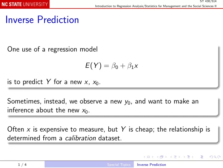
ST 430/514 Introduction to Regression Analysis/Statistics for Management and the Social Sciences II Inverse Prediction One use of a regression model E ( Y ) = β 0 + β 1 x is to predict Y for a new x , x 0 . Sometimes, instead, we observe a new y 0 , and want to make an inference about the new x 0 . Often x is expensive to measure, but Y is cheap; the relationship is determined from a calibration dataset. 1 / 4 Special Topics Inverse Prediction

ST 430/514 Introduction to Regression Analysis/Statistics for Management and the Social Sciences II Because y 0 = β 0 + β 1 x 0 + ǫ 0 , we can solve for x 0 : x 0 = y 0 − β 0 − ǫ 0 . β 1 We do not observe ǫ 0 , but we know that E ( ǫ 0 ) = 0. Similarly, we do not know β 0 and β 1 , but we have estimates ˆ β 0 and ˆ β 1 . 2 / 4 Special Topics Inverse Prediction

ST 430/514 Introduction to Regression Analysis/Statistics for Management and the Social Sciences II This suggests the estimate x 0 = y 0 − ˆ β 0 ˆ . ˆ β 1 This is known as inverse prediction . An approximate 100(1 − α )% prediction interval for x 0 is: � x ) 2 x 0 ± t α/ 2 × s 1 + 1 n + (ˆ x − ¯ ˆ . × ˆ SS xx β 1 3 / 4 Special Topics Inverse Prediction

ST 430/514 Introduction to Regression Analysis/Statistics for Management and the Social Sciences II An alternative approach is to fit the inverse regression : x = γ 0 + γ 1 y + ǫ. Then use the standard prediction interval � 1 + 1 n + ( y 0 − ¯ y ) 2 ˆ x 0 ± t α/ 2 × s x | y × SS yy where x 0 = ˆ ˆ γ 0 + ˆ γ 1 y 0 . This is not supported by the standard theory, because, in the calibration data, x is fixed and y is random. But it has been shown to work well in practice. 4 / 4 Special Topics Inverse Prediction