Introduction to the R Statistical Computing Environment R - PDF document

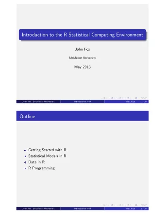
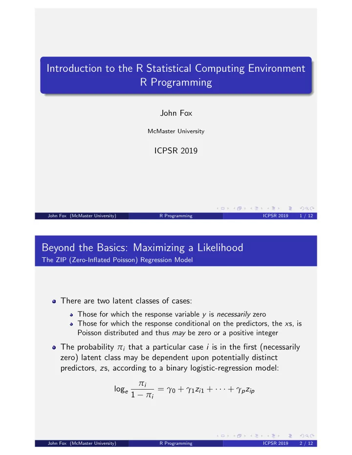
Introduction to the R Statistical Computing Environment R Programming John Fox McMaster University ICPSR 2019 John Fox (McMaster University) R Programming ICPSR 2019 1 / 12 Beyond the Basics: Maximizing a Likelihood The ZIP (Zero-Inflated Poisson) Regression Model There are two latent classes of cases: Those for which the response variable y is necessarily zero Those for which the response conditional on the predictors, the x s, is Poisson distributed and thus may be zero or a positive integer The probability π i that a particular case i is in the first (necessarily zero) latent class may be dependent upon potentially distinct predictors, z s, according to a binary logistic-regression model: π i = γ 0 + γ 1 z i 1 + · · · + γ p z ip log e 1 − π i John Fox (McMaster University) R Programming ICPSR 2019 2 / 12

Beyond the Basics: Maximizing a Likelihood The ZIP (Zero-Inflated Poisson) Regression Model For an individual i in the second latent class, y follows a Poisson regression model with log link, log e µ i = β 0 + β 1 x i 1 + · · · + β k x ik where µ i = E ( y i ) , and conditional distribution p ( y i | x 1 , . . . , x k ) = µ y i i e − µ i for y i = 0, 1, 2, . . . y i ! John Fox (McMaster University) R Programming ICPSR 2019 3 / 12 Beyond the Basics: Maximizing a Likelihood The ZIP (Zero-Inflated Poisson) Regression Model The probability of observing a zero count for case i , not knowing to which latent class the case belongs, is therefore p ( 0 ) = Pr ( y i = 0 ) = π i + ( 1 − π i ) e − µ i and the probability of observing a particular nonzero count y i > 0 is p ( y i ) = ( 1 − π i ) µ y i i e − µ i y i ! John Fox (McMaster University) R Programming ICPSR 2019 4 / 12

Beyond the Basics: Maximizing a Likelihood The ZIP (Zero-Inflated Poisson) Regression Model The log-likelihood for the ZIP model combines the two components, for y = 0 and for y > 0: π i + ( 1 − π i ) e − µ i � ∑ � log e ( β , γ ) = log e y i = 0 ( 1 − π i ) µ y i i e − µ i � � + ∑ log e y i ! y 1 > 0 where β = ( β 0 , β 1 , . . . , β k ) ′ is the vector of parameters from the Poisson-regression component of the model (on which the µ i depend) γ = ( γ 0 , γ 1 , . . . , γ p ) ′ is the vector of parameters from the logsitic-regression component of the model (on which the π i depend) John Fox (McMaster University) R Programming ICPSR 2019 5 / 12 Beyond the Basics: Maximizing a Likelihood The ZIP (Zero-Inflated Poisson) Regression Model In maximizing the likelihood, it helps (but isn’t essential) to have the gradient (vector of partial derivatives with respect to the parameters) of the log-likelihood. For the ZIP model the gradient is complicated: exp [ − exp ( x ′ i β )] exp ( x ′ ∂ log L ( β , γ ) i β ) = − ∑ i β )] x i exp ( z ′ i γ ) + exp [ − exp ( x ′ ∂ β i : y i = 0 + ∑ [ y i − exp ( x ′ i β )] x i i : y i > 0 exp ( z ′ ∂ log L ( β , γ ) i γ ) = ∑ i β )] z i exp ( z ′ i γ ) + exp [ − exp ( x ′ ∂ γ i : y i = 0 n exp ( z ′ i γ ) ∑ − i γ ) z i 1 + exp ( z ′ i = 1 John Fox (McMaster University) R Programming ICPSR 2019 6 / 12

Beyond the Basics: Maximizing a Likelihood The ZIP (Zero-Inflated Poisson) Regression Model And the Hessian (the matrix of second-order partial derivatives, from which the covariance matrix of the coefficients is computed) is even more complicated (thankfully we won’t need it): ∂ log L ( β , γ ) = ∂ β ∂ β ′ � � exp ( x ′ i β ) [ exp ( x ′ exp ( 2 x ′ i β ) − 1 ] i β ) x i x ′ ∑ i γ ] + 1 − exp [ exp ( x ′ i β ) + z ′ i i γ ] + 1 } 2 { exp [ exp ( x ′ i β ) + z ′ i : y i = 0 − ∑ exp ( x ′ i β ) x i x ′ i i : y i > 0 John Fox (McMaster University) R Programming ICPSR 2019 7 / 12 Beyond the Basics: Maximizing a Likelihood The ZIP (Zero-Inflated Poisson) Regression Model (Hessian continued): exp [ exp ( x ′ i β ) + z ′ ∂ log L ( β , γ ) i γ ] = ∑ i γ ] + 1 } 2 z i z ′ i ∂ γ ∂ γ ′ { exp [ exp ( x ′ i β ) + z ′ i : y i = 0 exp ( z ′ n i γ ) i γ ) + 1 ] 2 z i z ′ ∑ − i [ exp ( z ′ i = 1 exp [ x ′ i β + exp ( x ′ i β ) + z ′ ∂ log L ( β , γ ) i γ ] = ∑ i γ ] + 1 } 2 x i z ′ i ∂ β ∂ γ ′ { exp [ exp ( x ′ i β ) + z ′ i : y i = 0 John Fox (McMaster University) R Programming ICPSR 2019 8 / 12

Beyond the Basics: Maximizing a Likelihood The ZIP (Zero-Inflated Poisson) Regression Model We can let a general-purpose optimizer do the work of maximizing the log-likelihood Optimizers work by evaluating the gradient of the ‘objective function’ (the log-likelihood) at the current estimates of the parameters, either numerically or analytically They iteratively improve the parameter estimates using the information in the gradient Iteration ceases when the gradient is sufficiently close to zero. The covariance matrix of the coefficients is the inverse of the matrix of second derivatives of the log-likelihood, called the Hessian , which measures curvature of the log-likelihood at the maximum There is generally no advantage in using an analytic Hessian during optimization John Fox (McMaster University) R Programming ICPSR 2019 9 / 12 Beyond the Basics: Maximizing a Likelihood The ZIP (Zero-Inflated Poisson) Regression Model I’ll use the optim() function to fit the ZIP model. It takes several arguments, including: par , a vector of start values for the parameters fn , the objective function to be minimized (in our case the negative of the log-likelihood), the first argument of which is the parameter vector; there may be other arguments gr (optional), the gradient, also a function of the parameter vector (and possibly of other arguments) ... (optional), any other arguments to be passed to fn and gr method , I’ll use "BFGS" hessian , set to TRUE to return the numerical Hessian at the solution See ?optim for details and other optional arguments John Fox (McMaster University) R Programming ICPSR 2019 10 / 12

Beyond the Basics: Maximizing a Likelihood The ZIP (Zero-Inflated Poisson) Regression Model optim() returns a list with several element, including: par , the values of the parameters that minimize the objective function value , the value of the objective function at the minimum convergence , a code indicating whether the optimization has converged: 0 means that convergence occurred hessian , a numerical approximation to the Hessian at the solution Again, see ?optim for details John Fox (McMaster University) R Programming ICPSR 2019 11 / 12 Beyond the Basics: Object-Oriented Programming The S3 Object System Three standard object-oriented programming systems in R: S3, S4, reference classes How the S3 object system works Method dispatch, for object of class "class" : generic( object ) = ⇒ generic. class ( object ) = ⇒ generic.default( object ) For example, summarizing an object mod of class "lm" : summary(mod) = ⇒ summary.lm(mod) Objects can have more than one class, in which case the first applicable method is used. For example, objects produced by glm() are of class c("glm", "lm") and therefore can inherit methods from class "lm" . Generic functions: generic < - function(object, other-arguments, ... ) UseMethod("generic") For example, summary < - function(object, ...) UseMethod("summary") John Fox (McMaster University) R Programming ICPSR 2019 12 / 12