Introduction to pinhole cameras Lesson given by S erard in the course - PowerPoint PPT Presentation
Introduction to pinhole cameras Lesson given by S erard in the course ebastien Pi Introduction aux techniques audio et vid eo (ULg, Pr. J.J. Embrechts) INTELSIG, Montefiore Institute, University of Li` ege, Belgium October 30,
Introduction to pinhole cameras Lesson given by S´ erard in the course ebastien Pi´ “Introduction aux techniques audio et vid´ eo” (ULg, Pr. J.J. Embrechts) INTELSIG, Montefiore Institute, University of Li` ege, Belgium October 30, 2013 1 / 21
Optics : the light travels along straight line segments The light travels along straight lines if one assumes a single material (air, glass, etc. ) and a single frequency. Otherwise . . . 2 / 21
Optics : behavior of a lens Assuming the Gauss’ assumptions, all light rays coming from the same direction converge to a unique point on the focal plane. 3 / 21
Optics : an aperture 4 / 21
Optics : a pinhole camera A pinhole camera is a camera with a very small aperture. The lens becomes completely useless. The camera is just a small hole. High exposure durations are needed due to the limited amount of light received. 5 / 21
What is a camera ? A camera is a function: point in the 3D world → pixel � � � � x y z u v → � � � � ( c ) → � � ( f ) → � � x y z x y z u v u v → � � in the world 3D Cartesian coordinate system x y z ◮ � ( c ) in the 3D Cartesian coordinate system located � x y z ◮ at the camera’s optical center (the hole), with the axis z ( c ) along its optical axis, and the axis y ( c ) pointing upperwards. � ( f ) in the 2D Cartesian coordinate system locate in the � u v ◮ focal plane � � u v in the 2D coordinate system screen or image ◮ 6 / 21
( x y z ) → ( x y z ) ( c ) y x ❅ ■ ❅ � ✒ � ❅ � ❅ � ✏✏✏✏✏✏✏✏✏✏✏✏✏✏✏✏✏ ✏ ✶ y ( c ) ❅ ❅ ❘ ❅ ✻ z − → t � � ✛ z ( c ) ❅ ❅ ❅ ❅ ❅ ❘ x ( c ) x ( c ) x t x y ( c ) = R 3 × 3 y + t y z ( c ) z t z 7 / 21
( x y z ) → ( x y z ) ( c ) x ( c ) x t x y ( c ) = R 3 × 3 y + t y z ( c ) z t z R is a matrix that gives the rotation from the world coordinate system to the camera coordinate system. The columns of R are the base vectors of the world coordinate system expressed in the camera coordinate system. In the following, we will assume that the two coordinate systems are orthonormal. In this case, we have R T R = I ⇔ R − 1 = R T . 8 / 21
( x y z ) ( c ) → ( u v ) ( f ) ❅ ✟ ✟✟✟✟✟✟✟✟✟✟✟✟✟✟✟✟✟✟ s ❅ ❅ ❅ s ❅ ❅ ✥ ✥✥✥✥✥✥✥✥✥✥✥✥✥✥✥✥✥✥ y ( c ) v ( f ) ❅ ❅ ❅ ❅ ✻ ✻ ❅ ❅ ❅ ❅ ✛ ❅ ❅ z ( c ) ❅ ❅ ❅ ❘ f ❅ ❘ ❅ x ( c ) u ( f ) ❅ ❅ ❅ ❅ ❅ ❅ ❅ ❅ 9 / 21
( x y z ) ( c ) → ( u v ) ( f ) We suppose that the image plane is orthogonal to the optical axis. We have : x ( c ) f u ( f ) = z ( c ) y ( c ) f v ( f ) = z ( c ) 10 / 21
( u v ) ( f ) → ( u v ) v ( f ) v ✻ ✍ ✂ ✲ ✂ ✂✂ ✂✂ v 0 u ( f ) ✂ ✂ ✂ ✂ ✂ ✂ ✂ ✂ ✂ ✂✂ ✂✂ ✂ ✂ ✂ ✂ ✂ ✂ ✂ ✂ ✂ ✂ ✂ ✂ ✂ ✂ ✂ ✂ ✂ ✂ ✂ ✂ ✂ ✂ θ ✻ 1 ✂ ✂ ✂ ✂ ✂ ✂ ✂ ❄ k v ✂ ✂ ✂ ✂ ✂ ✂ ✂ ✂ ✂ ✂ ✂ ✂ ✂ ✂ ✲ u ✛ ✲ u 0 1 k u 11 / 21
( u v ) ( f ) → ( u v ) We have : u = ( u ( f ) − v ( f ) v = v ( f ) k v + v 0 tan θ ) k u + u 0 The parameters k u and k v are scaling factors and ( u 0 , v 0 ) are the coordinates of the point where the optical axis crosses the image plane. We pose s uv = − k u tan θ and obtain: su ( f ) su k u s uv u 0 sv ( f ) = 0 sv k v v 0 s 0 0 1 s Often, the grid of photosensitive cells can be considered as nearly rectangular. The parameter s uv is then neglected and is considered as 0. 12 / 21
The complete pinhole camera model With homogeneous coordinates the pinhole model can be written as a linear relation: t x x su k u s uv u 0 f 0 0 0 R 3 × 3 t y y sv = 0 k v v 0 0 f 0 0 t z z s 0 0 1 0 0 1 0 0 0 0 1 1 t x x 0 su α u S uv u 0 R 3 × 3 t y y sv = 0 v 0 0 α v ⇔ t z z s 0 0 1 0 0 0 0 1 1 x su m 11 m 12 m 13 m 14 y sv = m 21 m 22 m 23 m 24 ⇔ z s m 31 m 32 m 33 m 34 1 with α u = f k u , α v = f k v , and S uv = f s uv . 13 / 21
Questions Question What is the physical meaning of the homogeneous coordinates ? Think about all concurrent lines intersection at the origin and the three first elements of the homogeneous coordinates with ( x y z ) on a sphere . . . Question How many degrees of freedom has M 3 × 4 ? ( m 31 m 32 m 33 ) is a unit vector since ( m 31 m 32 m 33 ) = ( r 31 r 32 r 33 ). 14 / 21
The calibration step: finding the matrix M 3 × 4 15 / 21
The calibration step: finding the matrix M 3 × 4 x su m 11 m 12 m 13 m 14 y = sv m 21 m 22 m 23 m 24 z s m 31 m 32 m 33 m 34 1 therefore m 11 x + m 12 y + m 13 z + m 14 u = m 31 x + m 32 y + m 33 z + m 34 m 21 x + m 22 y + m 23 z + m 24 v = m 31 x + m 32 y + m 33 z + m 34 and ( m 31 u − m 11 ) x + ( m 32 u − m 12 ) y + ( m 33 u − m 13 ) z + ( m 34 u − m 14 ) = 0 ( m 31 v − m 21 ) x + ( m 32 v − m 22 ) y + ( m 33 v − m 23 ) z + ( m 34 v − m 24 ) = 0 16 / 21
The calibration step: finding the matrix M 3 × 4 m 11 m 12 x 1 y 1 z 1 1 0 0 0 0 − u 1 x 1 − u 1 y 1 − u 1 z 1 − u 1 m 13 1 0 0 0 0 x 2 y 2 z 2 − u 2 x 2 − u 2 y 2 − u 2 z 2 − u 2 m 14 . . . . . . . . . . . . . . . . . . . . . . . . . . . . . . . . . . . . m 21 1 0 0 0 0 x n y n z n − u n x n − u n y n − u n z n − u n m 22 = 0 0 0 0 0 x 1 y 1 z 1 1 − v 1 x 1 − v 1 y 1 − v 1 z 1 − v 1 m 23 0 0 0 0 1 x 2 y 2 z 2 − v 2 x 2 − v 2 y 2 − v 2 z 2 − v 2 m 24 . . . . . . . . . . . . m 31 . . . . . . . . . . . . . . . . . . . . . . . . m 32 0 0 0 0 1 x n y n z n − v n x n − v n y n − v n z n − v n m 33 m 34 17 / 21
Questions Question What is the minimum value for n ? 5 . 5 Question How can we solve the homogeneous system of the previous slide ? Apply a SVD and use the vector of the matrix V corresponding the smallest singular value. Question Is there a conditions on the set of 3D points used for calibrating the camera ? Yes, they should not be coplanar. 18 / 21
Intrinsic and extrinsic parameters m 11 m 12 m 13 m 14 α u S uv u 0 t x = 0 m 21 m 22 m 23 m 24 α v v 0 R 3 × 3 t y m 31 m 32 m 33 m 34 0 0 1 t z � �� � � �� � intrinsic parameters extrinsic parameters The decomposition can be achieved via the orthonormalising theorem of Graham-Schmidt, or via a QR decomposition since m 11 m 12 m 13 S uv u 0 r 11 r 12 r 13 α u m 21 m 22 m 23 = 0 α v v 0 r 21 r 22 r 23 m 31 m 32 m 33 0 0 1 r 31 r 32 r 33 m 33 m 23 m 13 r 33 r 23 r 13 1 v 0 u 0 = 0 m 32 m 22 m 12 r 32 r 22 r 12 α v S uv ⇔ m 31 m 21 m 11 r 31 r 21 r 11 0 0 α u 19 / 21
Questions Question What is the minimum of points to use for recalibrating a camera that has moved ? 3 since there are 6 degrees of freedom in the extrinsic parameters. Question What is this ? 20 / 21
Bibliography D. Forsyth and J. Ponce, Computer Vision: a Modern Approach . Prentice Hall, 2003. R. Hartley and A. Zisserman, Multiple View Geometry in Computer Vision , 2nd ed. Cambridge University Press, 2004. Z. Zhang,“A flexible new technique for camera calibration,” IEEE Transactions on Pattern Analysis and Machine Intelligence , vol. 22, no. 11, pp. 1330–1334, 2000. 21 / 21
Recommend
More recommend
Explore More Topics
Stay informed with curated content and fresh updates.


