Introducing Bayes Rasmus Bth, rasmus.baath@gmail.com King Digital - PowerPoint PPT Presentation
? Introducing Bayes Rasmus Bth, rasmus.baath@gmail.com King Digital Entertainment Some ways to introduce Bayes The base rate fallacy. You test positive, whats the probability you have this horrible rare disease? Not
? Introducing Bayes Rasmus Bååth, rasmus.baath@gmail.com King Digital Entertainment
Some ways to introduce Bayes ● The base rate fallacy. “You test positive, what’s the probability you have this horrible rare disease?” ○ Not statistics, no estimation. It’s only about Bayes rule. ● Mathematical with conjugate priors. “The data is Normally distributed with known standard deviation.” ○ When was ever the standard deviation known!? Fine if you like math, I guess. ● Personal belief and hypothesis testing. ○ Gets philosophical too fast! Why is the prior personal, but not the model? Does this model really update my personal prior, why can’t I just do it myself by just looking at the data? How do I know what my prior is?!
Introducing Bayes as conditioning with probability distributions represented by samples Not the greatest name perhaps...
We want to know ● How many visitors / clicks will we get out of a 100 shown adds. ● Will we get more than 5 clicks / visitors?
10%
A function simulating people clicking on 100 ads with an underlying rate of Binomial 10% distribution
n_visitors <- rbinom( n = 100000, size = 100, prob = 0.1) hist( n_visitors ) mean( n_visitors > 5) [1] 0.94
Done so far ➔ Represented uncertainty over future data with probability ➔ Worked with samples
n_visitors <- rbinom( n = 100000, size = 100, prob = 0.1) hist( n_visitors ) mean( n_visitors > 5) [1] 0.94
proportion_clicks <- runif( n = 100000, min = 0.0, max = 0.2) n_visitors <- rbinom( n = 100000, size = 100, prob = 0.1)
proportion_clicks <- runif( n = 100000, min = 0.0, max = 0.2) n_visitors <- rbinom( n = 100000, size = 100, prob = proportion_clicks )
proportion_clicks <- runif( n = 100000, min = 0.0, max = 0.2) n_visitors <- rbinom( n = 100000, size = 100, prob = proportion_clicks ) hist( n_visitors )
proportion_clicks <- runif( n = 100000, min = 0.0, max = 0.2) n_visitors <- rbinom( n = 100000, size = 100, prob = proportion_clicks ) hist( n_visitors ) mean( n_visitors > 5) [1] 0.70
Done so far ➔ Represented uncertainty over future data with probability ➔ Worked with samples ➔ Represented prior uncertainty over parameters with probability ➔ Produced a prior predictive distribution over future data
13× 100 “Now we just condition on this data!”
prior <- data.frame( proportion_clicks , n_visitors ) head( prior ) proportion_clicks n_visitors 1 0.20 20 2 0.07 6 3 0.07 8 4 0.06 6 5 0.01 1 6 0.05 2 plot( prior )
prior <- data.frame( proportion_clicks , n_visitors ) posterior <- prior [ prior$n_visitors == 13, ] hist( posterior$proportion_clicks ) n_visitors <- rbinom( n = 100000, size = 100, prob = posterior$proportion_clicks ) mean( n_visitors > 5) [1] 0.97
Done so far ➔ Represented uncertainty over future data with probability ➔ Worked with samples ➔ Represented prior uncertainty over parameters with probability ➔ Produced a prior predictive distribution over future data ➔ Bayesian inference by conditioning on the data ➔ Produced a posterior predictive distribution
Posterior Prior Posterior Prior Predictive Predictive
What’s bad What’s good ● No explicit mention of probability ● Applied example ● You never see Bayes rule ● Focus on getting a grip on ● The computational method uncertainty doesn’t scale to other models ● Everything is there: Priors, ● Of course, a one semester posteriors, samples, prediction, course would be better data, Bayesian updating! ● You build it up from scratch ● It’s crappy model, but it’s slightly less crap in the end.
“Statistical modeling is not about building the perfect true model. It’s about building a less crappy one.”
? Introducing Bayes Rasmus Bååth, rasmus.baath@gmail.com King Digital Entertainment
visitor_prob <- dbinom( x = 0 : 100, size = 100, prob = 0.1) plot(0 : 100, visitor_prob )
Recommend
More recommend
Explore More Topics
Stay informed with curated content and fresh updates.
