Generalized Bayesian Inference with Sets of Conjugate Priors for - PDF document

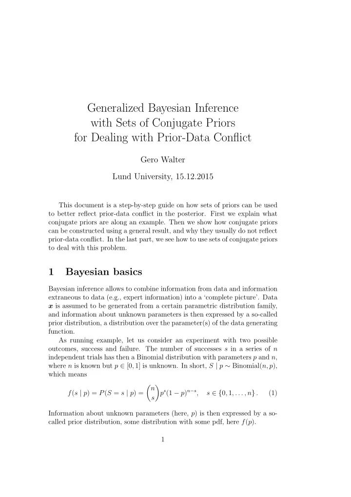
Generalized Bayesian Inference with Sets of Conjugate Priors for Dealing with Prior-Data Conflict Gero Walter Lund University, 15.12.2015 This document is a step-by-step guide on how sets of priors can be used to better reflect prior-data conflict in the posterior. First we explain what conjugate priors are along an example. Then we show how conjugate priors can be constructed using a general result, and why they usually do not reflect prior-data conflict. In the last part, we see how to use sets of conjugate priors to deal with this problem. 1 Bayesian basics Bayesian inference allows to combine information from data and information extraneous to data (e.g., expert information) into a ‘complete picture’. Data x is assumed to be generated from a certain parametric distribution family, and information about unknown parameters is then expressed by a so-called prior distribution, a distribution over the parameter(s) of the data generating function. As running example, let us consider an experiment with two possible outcomes, success and failure. The number of successes s in a series of n independent trials has then a Binomial distribution with parameters p and n , where n is known but p ∈ [0 , 1] is unknown. In short, S | p ∼ Binomial( n, p ), which means � n � p s (1 − p ) n − s , f ( s | p ) = P ( S = s | p ) = s ∈ { 0 , 1 , . . . , n } . (1) s Information about unknown parameters (here, p ) is then expressed by a so- called prior distribution, some distribution with some pdf, here f ( p ). 1

The ‘complete picture’ is then the so-called posterior distribution, here with pdf f ( p | s ), expressing the state of knowledge after having seen the data. It encompasses information from the prior f ( p ) and data and is ob- tained via Bayes’ Rule, f ( s | p ) f ( p ) d p = f ( s | p ) f ( p ) f ( s | p ) f ( p ) f ( p | s ) = ∝ f ( s | p ) f ( p ) , (2) � f ( s ) where f ( s ) is the so-called marginal distribution of the data S . In general, the posterior distribution is hard to obtain, especially due to the integral in the denominator. The posterior can be approximated with numerical methods, like the Laplace approximation or simulation methods like MCMC (Markov chain Monte Carlo). There is a large literature deal- ing with computations of posteriors, and software like BUGS or JAGS has been developed which simplifies the creation of a sampler to approximate a posterior. 2 A conjugate prior However, Bayesian inference not necessarily entails complex calculations and simulation methods. With a clever choice of parametric family for the prior distribution, the posterior distribution belongs to the same parametric family as the prior, just with updated parameters. Such prior distributions are called conjugate priors. Basically, with conjugate priors one trades flexibility for tractability: The parametric family restricts the form of the prior pdf, but with the advantage of much easier computations. 1 The conjugate prior for the Binomial distribution is the Beta distribution, which is usually parametrised with parameters α and β . 1 B ( α, β ) p α − 1 (1 − p ) β − 1 , f ( p | α, β ) = (3) where B ( · , · ) is the Beta function. 2 In short, we write p ∼ Beta( α, β ). From now on, we will denote prior parameter values by an upper index (0) , and updated, posterior parameter values by an upper index ( n ) . With this notational convention, let S | p ∼ Binomial( n, p ) and p ∼ Beta( α (0) , β (0) ). 1 In fact, practical Bayesian inference was mostly restricted to conjugate priors before the advent of MCMC. � 1 0 t a − 1 (1 − t ) b − 1 d t and gives the inverse 2 The Beta function is defined as B ( a, b ) = normalisation constant for the Beta distribution. It is related to the Gamma function through B ( a, b ) = Γ( a )Γ( b ) Γ( a + b ) . We will not need to work with Beta functions here. 2

Then it holds that p | s ∼ Beta( α ( n ) , β ( n ) ), where α ( n ) and β ( n ) are updated, posterior parameters, obtained as α ( n ) = α (0) + s , β ( n ) = β (0) + n − s . (4) From this we can see that α (0) and β (0) can be interpreted as pseudocounts, forming a hypothetical sample with α (0) sucesses and β (0) failures. Exercise 1. Confirm Eq. (4) , i.e., show that, when S | p ∼ Binomial( n, p ) and p ∼ Beta( α (0) , β (0) ) , the density of the posterior distribution for p is of the form Eq. (3) but with updated parameters. (Hint: use the last expression in Eq. (2) and consider for the posterior the terms related to p only.) You have seen in the talk that we considered a different parametrisation of the Beta distribution in terms of n (0) and y (0) , defined as α (0) n (0) = α (0) + β (0) , y (0) = α (0) + β (0) , (5) such that writing p ∼ Beta( n (0) , y (0) ) corresponds to f ( p | n (0) , y (0) ) = p n (0) y (0) − 1 (1 − p ) n (0) (1 − y (0) ) − 1 . (6) B ( n (0) y (0) , n (0) (1 − y (0) )) In this parametrisation, the updated, posterior parameters are given by n (0) n (0) + n · s n n ( n ) = n (0) + n , y ( n ) = n (0) + n · y (0) + n , (7) and we write p | s ∼ Beta( n ( n ) , y ( n ) ). Exercise 2. Confirm the equations for updating n (0) to n ( n ) and y (0) to y ( n ) . (Hint: Find expressions for α (0) and β (0) in terms of n (0) and y (0) , then use Eq. (4) and solve for n ( n ) and y ( n ) .) From the properties of the Beta distribution, it follows that y (0) = α (0) α (0) + β (0) = E[ p ] is the prior expectation for the success probability p , and that the higher n (0) , the more probability weight will be concentrated around y (0) , y (0) (1 − y (0) ) as Var( p ) = . From the interpretation of α and β and Eq. (5), n (0) +1 we see that n (0) can also be interpreted as a (total) pseudocount or prior strength. Exercise 3. Write a function dbetany(x,n,y, ...) that returns the value of the Beta density function at x for parameters n (0) and y (0) instead of shape1 ( = α ) and shape2 ( = β ) as in dbeta(x, shape1, shape2, ...) . Use your function to plot the Beta pdf for different values of n (0) and y (0) to see how the pdf changes according to the parameter values. 3

The formula for y ( n ) in Eq. (7) is not written in the most compact form in order to emphasize that y ( n ) , the posterior expectation of p , is a weighted average of the prior expectation y (0) and s/n (the fraction of successes in the data), with the weights n (0) and n , respectively. We see that n (0) plays the same role for the prior mean y (0) as the sample size n for the observed mean s/n , reinforcing the interpretation as pseudocount. Indeed, the higher n (0) , the higher the weight for y (0) in the weighted average calculation of y ( n ) , so n (0) gives the strength of the prior as compared to the sample size n . Exercise 4. Give a ceteris paribus analysis for E[ p | s ] = y ( n ) and Var( p | s ) = y ( n ) (1 − y ( n ) ) (i.e, discuss how E[ p | x ] and Var( p | s ) behave) when n ( n ) +1 (i) n (0) → 0 , (ii) n (0) → ∞ , and (iii) n → ∞ when s/n = const. and consider also the form of f ( p | s ) based on E[ p | s ] and Var( p | s ) . 3 Conjugate priors for canonical exponential families Fortunately it is not necessary to search or guess to find a conjugate prior to a certain data distribution, as there is a general result on how to construct conjugate priors when the sample distribution belongs to a so-called canon- ical exponential family (e.g., Bernardo and Smith 2000, pp. 202 and 272f). This result covers many sample distributions, like Normal and Multinomial models, Poisson models, or Exponential and Gamma models, and gives a common structure to all conjugate priors constructed in this way. For the construction, we will consider distributions of i.i.d. samples x = ( x 1 , . . . , x n ) of size n directly. 3 With the Binomial distribution, we did so indirectly only: The Binomial( n, p ) distribution for S results from n inde- pendent trials with success probability p each. Encoding success as x i = 1 and failure as x i = 0 and collecting the n results in a vector x , we get s = � n i =1 x i . It turns out that the sample distribution depends on x only 3 It would be possible, and indeed is often done in the literature, to consider a single observation x in Eq. (9) only, as the conjugacy property does not depend on the sample size. However, we find our version with n -dimensional i.i.d. sample x more appropriate. 4