Intrinsic Images by Entropy Minimization How Peter Pan Really Lost - PowerPoint PPT Presentation

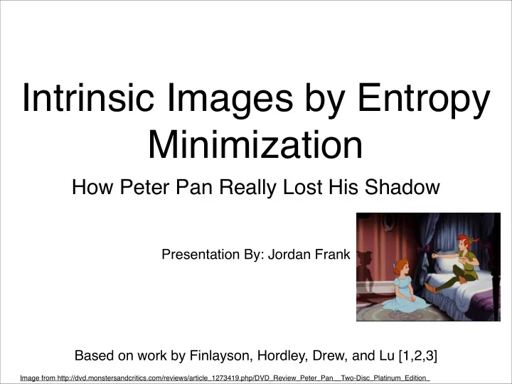
Intrinsic Images by Entropy Minimization How Peter Pan Really Lost His Shadow Presentation By: Jordan Frank Based on work by Finlayson, Hordley, Drew, and Lu [1,2,3] Image from http://dvd.monstersandcritics.com/reviews/article_1273419.php/DVD_Review_Peter_Pan__Two-Disc_Platinum_Edition_

Colour Constancy • Humans automatically remove the effect of lighting in visual perception. Our vision system is very robust to illumination. • We can easily tell that the bricks in the sunlight are the same colour as the bricks in the shade.

Colour Constancy • However, this is an Ill-posed problem. • We cannot tell whether differences in the colour that we detect are due to differences in the colour of the object, or differences in illumination. • What if the bricks on the right really were darker? In fact, there are small differences in the colours, even within a single brick.

Invariant Image • Goal is to produce an image that is invariant to effects of illumination. • Motivation: • Add our own illumination. • Remove shadows! Almost every presentation prior to this one has talked about how shadows are problematic.

Cameras/Sensors • RGB colour at a pixel results from an integral over the visible wavelength � R k = σ E ( λ ) S ( λ ) Q k ( λ ) d λ , k = R, G, B (1) σ – Lambertian shading E ( λ ) – illumination spectral power distribution S ( λ ) – surface spectral reflectance Q k ( λ ) – camera sensitivity

Cameras/Sensors • For convenience we assume that camera sensitivity is exactly a Dirac delta function Q k ( λ ) = q k δ ( λ − λ k ) • is the strength of the sensor. q k = Q k ( λ k ) • So (1) reduces to R k = σ E ( λ k ) S ( λ k ) q k

More Approximations • Supposing that lighting can be approximated by Planck ’ s law, with Wien ’ s approximation [4] we get k e − k 2 R k = σ Ik 1 λ − 5 T λ S ( λ k ) q k (2) • k 1 , k 2 are constants, temperature T characterizes the lighting colour and I gives the overall light intensity.

Removing I and σ • We can effectively remove the effect of Lambertian shading and illumination from (2) by dividing to get the band-ratio 2-vector chromaticities c , c k = R k /R p , where p is one of the channels and k= 1,2 indexes over the remaining responses.

Log Chromaticities • Log chromaticities are independent of illumination intensity, and translate under change of illumination colour. • (ln R / G ,ln B / G ) under one light becomes (ln R / G ,ln B / G )+( a , b ) under a second light. • More importantly, the translational term for different illuminants can always be written as ( α a , α b ) where a , b are constants and α depends on illumination.

Invariance, finally • Illumination change translates log chromaticities in the same direction. • Therefore, the coordinate axis orthogonal to the direction of illumination variation, y = - ( a / b ) x , records only illuminant invariant information.

Example (simulated) Measured log chromaticities After rotation Fig. 6. Perfect Dirac delta camera data (sensitivities anchored Fig. 7. Perfect Dirac delta camera data (sensitivities anchored Figures from [3]

Great in theory, but... • There are a number of problems with this approach. • Cameras do not have Dirac delta responses. • Noise! • How do we determine how much to rotate.

Narrowband, not Dirac Actual measurements from a SONY DXC-930 camera Rotated So we are still doing pretty well. Figures from [3]

How to calibrate • We can carefully calibrate our cameras to determine the best rotation angle through inspection of log chromaticities. 0 0.2 − 0.2 0 − 0.4 − 0.2 − 0.6 − 0.4 log(B/G) log(B/G) − 0.8 − 0.6 − 1 − 0.8 − 1.2 − 1 − 1.4 − 1.2 − 1.6 − 1.4 − 0.4 − 0.2 0 0.2 0.4 0.6 0.8 1 1.2 1.4 − 0.8 − 0.6 − 0.4 − 0.2 0 0.2 0.4 0.6 0.8 1 log( R/G) log(R/G) (a) (b) (c) Fig. 2. (a): Macbeth ColorChecker Chart image under a Planckian light. (b): Log-chromaticities of the 24 patches. (c): Median chromaticities for 6 patches, imaged under 14 different Planckian illuminants. Figure and caption from [1]

How to calibrate • Manual calibration is time-consuming, and requires numerous images under various lighting conditions. • We would like to find a way to find the desired parameters from just one image, without even knowing the camera that was used.

Intuition Greyscale image Greyscale image Invariant direction Wrong invariant direction log(B/R) log(B/R) log(G/R) log(G/R) And so what might be a good way to determine the best invariant direction? (Hint: we learned about it in this course) Figures from [1]

Entropy to the Rescue Greyscale image Greyscale image Invariant direction Wrong invariant direction log(B/R) log(B/R) log(G/R) log(G/R) Low Entropy High Entropy Figures from [1]

Entropy Minimization Algorithm : 1. Form a 2D log-chromaticity representation of the image. 2. for θ = 1..180 a) Rotate by θ and take projection onto x - axis b) Calculate entropy c) Keep track of θ that minimizes entropy

Problems/Solutions • How to calculate entropy? Solution: Create a histogram, compute bin widths using Scott ’ s Rule: bin_width = 3.49 std (projected_data) N 1/3 • Noise in the data? Solution: Use only the middle 90% of the projected data. • How to go back from rotated data to a usable image? Solution: See the paper, not easy!

Problems/Solutions • How to calculate entropy? Solution: Create a histogram, compute bin widths using Scott ’ s Rule: bin_width = 3.49 std (projected_data) N 1/3 • Noise in the data? Solution: Use only the middle 90% of the projected data. • How to go back from rotated data to a usable image? Solution: See the paper, not easy!

Problems/Solutions • How to calculate entropy? Solution: Create a histogram, compute bin widths using Scott ’ s Rule: bin_width = 3.49 std (projected_data) N 1/3 • Noise in the data? Solution: Use only the middle 90% of the projected data. • How to go back from rotated data to a usable image? Solution: See the paper, not easy!

Problems/Solutions • How to calculate entropy? Solution: Create a histogram, compute bin widths using Scott ’ s Rule: bin_width = 3.49 std (projected_data) N 1/3 • Noise in the data? Solution: Use only the middle 90% of the projected data. • How to go back from rotated data to a usable image? Solution: See the paper, not easy!

Example Original Image 6 5.5 Entropy Min-Entropy Projection 5 4.5 4 0 50 100 150 200 Angle Figures from [1]

Removing Shadows • Now that we have an image without shadows, how can we use this to remove shadows from the original image? Image from http://collectibles.about.com/library/priceguides/blpgDSpeterpan903.htm

Removing Shadows • Need to reintegrate the illumination invariant image into the original image. • Create an edge map for the Mean-Shift processed original image as well as the invariant image. • If the magnitude of the gradient in the invariant image is close to zero where the gradient in log response in the original image is high, then this is evidence of a shadow edge.

Removing Shadows Left to right, Edges in the original image, edges in the invariant image, recovered shadow edge. Figures from [2]

Removing Shadows • All edges in the image that are not shadow edges are indicative of material changes. There are no sharp changes due to illumination and so shadows have been removed. • Reintegrating the gradient gives a log response image which does not have shadows. For details, see the paper. • To get back to a realistic image, we simply have to add artificial illumination.

Results (Paper) 6.4 6.2 6 5.8 Entropy 5.6 5.4 5.2 5 4.8 0 20 40 60 80 100 120 140 160 180 Angle 12.5 12 Entropy 11.5 11 0 20 40 60 80 100 120 140 160 180 Angle 6.45 6.4 6.35 6.3 6.25 Entropy 6.2 6.15 6.1 6.05 6 5.95 0 20 40 60 80 100 120 140 160 180 Angle Figures from [3]

Results (Paper) 4.6 4.4 4.2 4 Entropy 3.8 3.6 3.4 3.2 0 20 40 60 80 100 120 140 160 180 Angle 7.75 7.7 7.65 7.6 7.55 Entropy 7.5 7.45 7.4 7.35 7.3 7.25 0 20 40 60 80 100 120 140 160 180 Angle 6 5.8 5.6 5.4 Entropy 5.2 5 4.8 4.6 4.4 0 20 40 60 80 100 120 140 160 180 Angle 4.8 4.75 4.7 4.65 4.6 Entropy 4.55 4.5 4.45 4.4 4.35 0 20 40 60 80 100 120 140 160 180 Angle Figures from [3]

Results (Mine) • The cameras that were used by the authors of the paper are professional quality. They claim in the paper that the methods work on all of the cameras that they tested, but the question is whether they actually tested consumer-grade cameras. • So I went out on a sunny day and snapped a few shots with my Pentax Optio WPi 6.0 megapixel camera.

Results (Mine) • My results weren ’ t quite as spectacular.

Results (Mine)

Questions? “If he thought at all, but I don't believe he ever thought, it was that he and his shadow, when brought near each other, would join like drops of water, and when they did not he was appalled. He tried to stick it on with soap from the bathroom, but that also failed. A shudder passed through Peter, and he sat on the floor and cried.” “Peter Pan : The Story of Peter and Wendy” J. M. Barrie