Interplay between statistical and deterministic methods Mihaela - PowerPoint PPT Presentation
Noise models for inverse problems Tikhonov regularization in Hilbert scales Regularized Newton methods Interplay between statistical and deterministic methods Mihaela Pricop, Frank Bauer Institute for Mathematical Stochastics University of
Noise models for inverse problems Tikhonov regularization in Hilbert scales Regularized Newton methods Interplay between statistical and deterministic methods Mihaela Pricop, Frank Bauer Institute for Mathematical Stochastics University of Göttingen Department for Knowledge-Based Mathematical Systems, Johannes Kepler University Linz Vienna 2009
Noise models for inverse problems Tikhonov regularization in Hilbert scales Regularized Newton methods Inverse problem Goal: To estimate a † ∈ X , not directly observable when u belonging to the separable Hilbert space Y is known and F : D ( F ) ⊂ X → Y F ( a † ) = u . F is a possibly nonlinear, injective operator. The problem is ill-posed in the sense that F − 1 is not continuous.
Noise models for inverse problems Tikhonov regularization in Hilbert scales Regularized Newton methods Definitions Definition A continuous linear operator ǫ : Y → L 2 (Ω , K , P ) is called a Hilbert-space process. The covariance cov ǫ : Y → Y of ǫ is the bounded operator defined by � cov ǫ φ 1 , φ 2 � = Cov ( � ǫ, φ 1 � , � ǫ, φ 2 � ) , φ 1 , φ 2 ∈ Y . Definition ǫ is a white noise process if cov ǫ = I . Every Hilbert-space valued random variable Σ with finite second moment can be identified with a Hilbert-space process by the operator Φ → � Φ , Σ � . A Gaussian white noise process in an infinite-dimensional Hilbert space can not be identified with a Hilbert-space valued random variable with finite second moment.
Noise models for inverse problems Tikhonov regularization in Hilbert scales Regularized Newton methods Abstract noise model Y = u + δξ + σǫ deterministic error ξ ∈ Y , � ξ � Y = 1 stochastic error ǫ is a Hilbert-space process with E � ǫ, φ � Y = 0, � cov ǫ � ≤ 1. Remark White noise models occur as limits of discrete noise models as the sample size n tends to infinity. 1 We have σ ∼ √ n . Brown & Low, 1996 Mathé & Pereverzev (2003) Bissantz, Hohage, Munk & Ruymgaart (2007)
Noise models for inverse problems Tikhonov regularization in Hilbert scales Regularized Newton methods Aims in inverse problems The discontinuous operator F − 1 is approximated by a family of continuous operators { R α : α > 0 } . We also need a parameter choice rule α = α ( Y , δ, σ ) to obtain an estimate � a = R α ( Y ,δ,σ ) ( Y ) . Convergence for deterministic errors � R α ( F ( a † )+ δξ,δ ) ( F ( a † ) + δξ ) − a † � δ → 0 sup − → 0 � ξ �≤ 1
Noise models for inverse problems Tikhonov regularization in Hilbert scales Regularized Newton methods Consistency for random noise � � σ → 0 � R α ( F ( a † )+ σǫ,σ ) ( F ( a † ) + σǫ ) − a † � 2 > θ P − → 0 , ∀ θ > 0 Quadratic risk for random noise E � R α ( F ( a † )+ σǫ,σ ) ( F ( a † ) + σǫ ) − a † � 2 σ → 0 − → 0 Probabilistic rates: ∀ σ ∃ t 1 ( σ ) σ → 0 → 0 , t 2 ( σ ) σ → 0 − − → 0 such that � � � R α ( F ( a † )+ σǫ,σ ) ( F ( a † ) + σǫ ) − a † � 2 ≥ t 1 ( σ ) P ≤ t 2 ( σ )
Noise models for inverse problems Tikhonov regularization in Hilbert scales Regularized Newton methods Rates of convergence For ill-posed problems, rates of convergence can only be obtained under further a-priori information on the solution, e.g. that a † belongs to a smoothness class S . Deterministic optimal rate � R α ( F ( a † )+ δξ,δ ) ( F ( a † ) + δξ ) − a † � △ ( δ, S , F ) = inf sup R � ξ �≤ 1 , a † ∈ S Statistical minimax risk � E � R α ( F ( a † )+ σǫ,σ ) ( F ( a † ) + σǫ ) − a † � 2 △ ( σ, S , F ) = inf R sup a † ∈ S
Noise models for inverse problems Tikhonov regularization in Hilbert scales Regularized Newton methods Oracle inequalities (stochastic) Oracle inequalities: E � R α ( F ( a † )+ σǫ,σ ) ( F ( a † ) + σǫ ) − a † � 2 ≤ � σ 2 � α E � R α ( F ( a † ) + σǫ ) − a † � 2 + O ρ σ inf Donoho & Johnstone 1994, Cavalier & Golubev & Picard & Tsybakov 2002
Noise models for inverse problems Tikhonov regularization in Hilbert scales Regularized Newton methods Oracle inequalities (deterministic) weak oracle inequality � � R α ( F ( a † )+ δξ,δ ) ( F ( a † )+ δξ ) − a † � ≤ C inf α sup � ξ �≤ 1 � R α ( F ( a † )+ � δξ ) − R α ( F ( a † )) � + � R α ( F ( a † )) − a † � + O ( δ ) strong oracle inequality � R α ( F ( a † )+ δξ,δ ) ( F ( a † ) + δξ ) − a † � ≤ α � R α ( F ( a † ) + δξ ) − a † � + O ( δ ) c sup inf ξ (Raus & Hämarik, recent papers) oracle inequality (Bauer, Kindermann 2008) � R α ( F ( a † )+ δξ,δ ) ( F ( a † ) + δξ ) − a † � ≤ � � � R α ( F ( a † ) + δξ ) − R α ( F ( a † )) � + � R α ( F ( a † )) − a † � C inf α
Noise models for inverse problems Tikhonov regularization in Hilbert scales Regularized Newton methods Oracle inequalities for linear inverse problems Deterministic/Deterministic: Knowing δ : deterministic oracle inequality (Lepski˘ ı balancing, Mathé & Pereverzev 2003, 2006) Restricted sets/saturation: oracle inequality (quasi-optimality, Bauer, Kindermann 2008) Deterministic/Stochastic: Knowing σ : oracle inequality loosing logarithmic factor (Lepski˘ ı balancing) Restricted sets/saturation: oracle inequality (quasi-optimality, Bauer, Kindermann 2008) Bayesian/Stochastic: Oracle inequality, even without knowing σ (quasi-optimality, Bauer, Reiß2008)
Noise models for inverse problems Tikhonov regularization in Hilbert scales Regularized Newton methods Nonlinear statistical inverse problems O’Sullivan 1990: first convergence rate result (suboptimal rates with restrictive assumptions) Bissantz & Hohage & Munk 2004: consistency and optimal rates for one smoothness class for Tikhonov regularization Hohage & Pricop 2008: optimal rates in a range of smoothness classes for Tikhonov regularization Bauer & Hohage & Munk 2009: convergence rates for regularized Newton method and optimal rates
Noise models for inverse problems Tikhonov regularization in Hilbert scales Regularized Newton methods 2-step method for nonlinear inverse problems F : X → Y is a nonlinear, injective operator. An estimator � u of u ∈ Y is chosen, Y a Hilbert space, such � u − u � 2 E � � that Y ≤ τ with known τ . a ∈ D ( F ) is an estimator of a † : � u � 2 Y + α � a − a 0 � 2 � a := argmin a ∈ D ( F ) {� F ( a ) − � X } Bissantz & Hohage & Munk 2004
Noise models for inverse problems Tikhonov regularization in Hilbert scales Regularized Newton methods Hilbert scales Consider an operator L : D ( L ) → X unbounded, self-adjoint, strictly positive, D ( L ) ⊂ X dense. X s := D ( L s ) , s ≥ 0, � x , y � s := � L s x , L s y � X , x , y ∈ X s For s < 0 we define X s as completion of X under the norm � x � s := < x , x > 1 / 2 s ( X s ) s ∈ R is the Hilbert scale induced by L Natterer 1984: Rates of convergence for deterministic linear inverse problems
Noise models for inverse problems Tikhonov regularization in Hilbert scales Regularized Newton methods Tikhonov regularization in Hilbert scales Nonlinear Inverse Problems � a is the solution of u � 2 Y + α � a − a 0 � 2 � F ( a ) − � s → min , a ∈ D ( F ) ∩ ( a 0 + X s ) Assumptions 1. D ( F ) is convex, F is continuous, injective, Fréchet-differentiable on X and weakly closed on X s for some s ≥ 0. 2. � F ′ ( a † ) h � Y ∼ � h � − p , ∀ h ∈ X , for some known p > 0. 3. There exists M > 0 such that a ∈ D ( F ) ∩ ( a 0 + X s ) � F ′ ( a † ) − F ′ ( a ) � Y←X − p ≤ M � a † − a 0 � 0 ≤ λ 2 Λ . Neubauer 1992: Deterministic convergence rate with � · � Y←X in Assumption 3.
Noise models for inverse problems Tikhonov regularization in Hilbert scales Regularized Newton methods A-priori choice of the regularization parameter Theorem (Hohage, Pricop) If the Assumptions 1 − 3 are fulfilled, a † − a 0 ∈ X q , 2 ( p + s ) q ∈ [ s , p + 2 s ] , s ≥ p and α ∼ τ then p + q � � 2 q a − a † � 2 E � � X = O τ . q + p For linear operators the upper bounds of the previous theorem agree with the minimax lower bound. For nonlinear operators lower bounds are not available and the upper bounds for the combined method are derived from case to case.
Noise models for inverse problems Tikhonov regularization in Hilbert scales Regularized Newton methods Convergence for Lepski˘ ı choice in deterministic setting Lepski˘ ı 1990: adaptive choice of the regularization parameter for regression problems Mathé, Pereverzev 2003 , 2006: the Lepski˘ ı principle for linear inverse problems We use the error splitting � a † − � a � ≤ � a † − a α � + � a α − � a � where � � � F ( a ) − F ( a † ) � 2 Y + α � a − a 0 � 2 a α := argmin a ∈ D ( F ) ∩ ( a 0 + X s ) . s Theorem (Pricop) Let Assumptions 1 − 3, a † − a 0 ∈ X q , q ∈ [ s , p + 2 s ] , s ≥ p and a deterministic noise model hold. Then it holds q � a α − a † � X ≤ C 1 α 2 ( p + s ) − p q 2 ( p + s ) + α 2 ( p + s ) ) � � a − a α � X ≤ c 1 ( δα with the constants C 1 and c 1 depending on a † , p , q , s .
Recommend
More recommend
Explore More Topics
Stay informed with curated content and fresh updates.
