Interest Points Computer Vision Jia-Bin Huang, Virginia Tech Many - - PowerPoint PPT Presentation

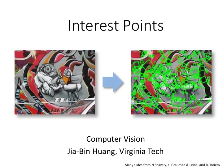
Interest Points

Computer Vision Jia-Bin Huang, Virginia Tech

Many slides from N Snavely, K. Grauman & Leibe, and D. Hoiem

Administrative Stuffs

• HW 1 posted, due 11:59 PM Sept 25
• Submission through Canvas
• Frequently Asked Questions for HW 1 will be

posted on piazza

• Reading - Szeliski: 4.1

What have we learned so far?

• Light and color

– What an image records

• Filtering in spatial domain
• Filtering = weighted sum of neighboring pixels
• Smoothing, sharpening, measuring texture
• Filtering in frequency domain
• Filtering = change frequency of the input image
• Denoising, sampling, image compression
• Image pyramid and template matching
• Filtering = a way to find a template
• Image pyramids for coarse-to-fine search and

multi-scale detection

• Edge detection
• Canny edge = smooth -> derivative -> thin ->

threshold -> link

• Finding straight lines, binary image analysis

This module: Correspondence and Alignment

• Correspondence:

matching points, patches, edges, or regions across images ≈

Slide credit: Derek Hoiem

This module: Correspondence and Alignment

• Alignment/registration:

solving the transformation that makes two things match better

Slide credit: Derek Hoiem

The three biggest problems in computer vision?

• 1. Registration
• 2. Registration
• 3. Registration

Takeo Kanade (CMU)

Example: automatic panoramas

Credit: Matt Brown

A

Example: fitting an 2D shape template

Slide from Silvio Savarese

Example: fitting a 3D object model

Slide from Silvio Savarese

Example: estimating “fundamental matrix” that corresponds two views

Slide from Silvio Savarese

Example: tracking points

frame 0 frame 22 frame 49 x x x

Today’s class

• What is interest point?
• Corner detection
• Handling scale and orientation
• Feature matching

Why extract features?

• Motivation: panorama stitching
• We have two images – how do we combine them?

Why extract features?

• Motivation: panorama stitching
• We have two images – how do we combine them?

Step 1: extract features Step 2: match features

Why extract features?

• Motivation: panorama stitching
• We have two images – how do we combine them?

Step 1: extract features Step 2: match features Step 3: align images

Image matching

by Diva Sian by swashford

Harder case

by Diva Sian by scgbt

Harder still?

NASA Mars Rover images with SIFT feature matches

Answer below (look for tiny colored squares…)

Applications

• Keypoints are used for:
• Image alignment
• 3D reconstruction
• Motion tracking
• Robot navigation
• Indexing and database retrieval
• Object recognition

Advantages of local features

Locality

• features are local, so robust to occlusion and clutter

Quantity

• hundreds or thousands in a single image

Distinctiveness:

• can differentiate a large database of objects

Efficiency

• real-time performance achievable

Overview of Keypoint Matching

• K. Grauman, B. Leibe

A

f

B

f

A1 A2 A3

T f f d

B A

< ) , (

• 1. Find a set of

distinctive key- points

• 3. Extract and

normalize the region content

• 2. Define a region

around each keypoint

• 4. Compute a local

descriptor from the normalized region

• 5. Match local

descriptors

Goals for Keypoints

Detect points that are repeatable and distinctive

Key trade-offs

More Repeatable More Points

A1 A2 A3

Detection

More Distinctive More Flexible

Description

Robust to occlusion Works with less texture Minimize wrong matches Robust to expected variations Maximize correct matches Robust detection Precise localization

Choosing interest points

Where would you tell your friend to meet you?

Choosing interest points

Where would you tell your friend to meet you?

Corner Detection: Basic Idea

“flat” region: no change in all directions “edge”: no change along the edge direction “corner”: significant change in all directions

• How does the window change when you shift it?
• Shifting the window in any direction causes a big

change

Credit: S. Seitz, D. Frolova, D. Simakov

Consider shifting the window W by (u,v)

• how do the pixels in W change?
• compare each pixel before and after by

summing up the squared differences (SSD)

• this defines an SSD “error” E(u,v):

Harris corner detection: the math

W

Taylor Series expansion of I: If the motion (u,v) is small, then first order approximation is good Plugging this into the formula on the previous slide…

Small motion assumption

Harris corner detection: the math

Using the small motion assumption, replace I with a linear approximation

W

(Shorthand: )

Corner detection: the math

W

• Thus, E(u,v) is locally approximated as a quadratic form

The surface E(u,v) is locally approximated by a quadratic form.

The second moment matrix

Let’s try to understand its shape.

Horizontal edge: u v E(u,v)

Vertical edge: u v E(u,v)

General case

The shape of H tells us something about the distribution

• f gradients around a pixel

We can visualize H as an ellipse with axis lengths determined by the eigenvalues of H and orientation determined by the eigenvectors of H

direction of the slowest change direction of the fastest change

(λmax)-1/2 (λmin)-1/2 const ] [ =       v u H v u Ellipse equation: λmax, λmin : eigenvalues of H

Quick eigenvalue/eigenvector review

The eigenvectors of a matrix A are the vectors x that satisfy: The scalar λ is the eigenvalue corresponding to x

• The eigenvalues are found by solving:
• In our case, A = H is a 2x2 matrix, so we have
• The solution:

Once you know λ, you find x by solving

Corner detection: the math

Eigenvalues and eigenvectors of H

• Define shift directions with the smallest and largest change in error
• xmax = direction of largest increase in E
• λmax = amount of increase in direction xmax
• xmin = direction of smallest increase in E
• λmin = amount of increase in direction xmin

xmin xmax

Corner detection: the math

How are λmax, xmax, λmin, and xmin relevant for feature detection?

• What’s our feature scoring function?

Corner detection: the math

How are λmax, xmax, λmin, and xmin relevant for feature detection?

• What’s our feature scoring function?

Want E(u,v) to be large for small shifts in all directions

• the minimum of E(u,v) should be large, over all unit vectors [u v]
• this minimum is given by the smaller eigenvalue (λmin) of H

Interpreting the eigenvalues

λ1 λ2 “Corner” λ1 and λ2 are large, λ1 ~ λ2; E increases in all

directions

λ1 and λ2 are small; E is almost constant

in all directions

“Edge” λ1 >> λ2 “Edge” λ2 >> λ1 “Flat” region

Classification of image points using eigenvalues of M:

Corner detection summary

Here’s what you do

• Compute the gradient at each point in the image
• Create the H matrix from the entries in the gradient
• Compute the eigenvalues.
• Find points with large response (λmin > threshold)
• Choose those points where λmin is a local maximum as features

Corner detection summary

Here’s what you do

• Compute the gradient at each point in the image
• Create the H matrix from the entries in the gradient
• Compute the eigenvalues.
• Find points with large response (λmin > threshold)
• Choose those points where λmin is a local maximum as features

The Harris operator

λmin is a variant of the “Harris operator” for feature detection

• The trace is the sum of the diagonals, i.e., trace(H) = h11 + h22
• Very similar to λmin but less expensive (no square root)
• Called the “Harris Corner Detector” or “Harris Operator”
• Lots of other detectors, this is one of the most popular

The Harris operator

Harris

• perator

Harris detector example

f value (red high, blue low)

Threshold (f > value)

Find local maxima of f

Harris features (in red)

Weighting the derivatives

• In practice, using a simple window W doesn’t work

too well

• Instead, we’ll weight each derivative value based
• n its distance from the center pixel

Harris Detector – Responses [Harris88]

Effect: A very precise corner detector.

Harris Detector – Responses [Harris88]

Harris Detector: Invariance Properties

• Rotation

Ellipse rotates but its shape (i.e. eigenvalues) remains the same Corner response is invariant to image rotation

Harris Detector: Invariance Properties

• Affine intensity change: I → aI + b

 Only derivatives are used => invariance to intensity shift I → I + b  Intensity scale: I → a I R x (image coordinate)

threshold

R x (image coordinate) Partially invariant to affine intensity change

Harris Detector: Invariance Properties

• Scaling

All points will be classified as edges Corner

Not invariant to scaling

Scale invariant detection

Suppose you’re looking for corners Key idea: find scale that gives local maximum of f

• in both position and scale
• One definition of f: the Harris operator

Automatic Scale Selection

• K. Grauman, B. Leibe

)) , ( ( )) , ( (

1 1

σ σ ′ ′ = x I f x I f

m m

i i i i  

How to find corresponding patch sizes?

Automatic Scale Selection

• Function responses for increasing scale (scale signature)
• K. Grauman, B. Leibe

)) , ( (

1

σ x I f

m

i i 

)) , ( (

1

σ x I f

m

i i

′



Automatic Scale Selection

• K. Grauman, B. Leibe

)) , ( (

1

σ x I f

m

i i 

)) , ( (

1

σ x I f

m

i i

′



• Function responses for increasing scale (scale signature)

Automatic Scale Selection

• K. Grauman, B. Leibe

)) , ( (

1

σ x I f

m

i i 

)) , ( (

1

σ x I f

m

i i

′



• Function responses for increasing scale (scale signature)

Automatic Scale Selection

• K. Grauman, B. Leibe

)) , ( (

1

σ x I f

m

i i 

)) , ( (

1

σ x I f

m

i i

′



• Function responses for increasing scale (scale signature)

Automatic Scale Selection

• K. Grauman, B. Leibe

)) , ( (

1

σ x I f

m

i i 

)) , ( (

1

σ x I f

m

i i

′



• Function responses for increasing scale (scale signature)

Automatic Scale Selection

• K. Grauman, B. Leibe

)) , ( (

1

σ x I f

m

i i 

)) , ( (

1

σ′ ′ x I f

m

i i 

• Function responses for increasing scale (scale signature)

Implementation

• Instead of computing f for larger and larger

windows, we can implement using a fixed window size with a Gaussian pyramid

(sometimes need to create in- between levels, e.g. a ¾-size image)

What Is A Useful Signature Function?

• Difference-of-Gaussian = “blob” detector
• K. Grauman, B. Leibe

Difference-of-Gaussian (DoG)

• K. Grauman, B. Leibe
• =

DoG – Efficient Computation

• Computation in Gaussian scale pyramid
• K. Grauman, B. Leibe

σ Original image

4 1

2 = σ

Sampling with step σ4 =2 σ σ σ

Find local maxima in position-scale space of Difference-of-Gaussian

• K. Grauman, B. Leibe

) ( ) ( σ σ

yy xx

L L +

σ σ2 σ3 σ4 σ5 ⇒ List st o

• f

(x, x, y y, , s)

Results: Difference-of-Gaussian

• K. Grauman, B. Leibe

• T. Tuytelaars, B. Leibe

Orientation Normalization

• Compute orientation histogram
• Select dominant orientation
• Normalize: rotate to fixed orientation

2π

[Lowe, SIFT, 1999]

Maximally Stable Extremal Regions [Matas ‘02]

• Based on Watershed segmentation algorithm
• Select regions that stay stable over a large

parameter range

• K. Grauman, B. Leibe

Example Results: MSER

73

• K. Grauman, B. Leibe

Available at a web site near you…

• For most local feature detectors, executables are

available online:

– http://www.robots.ox.ac.uk/~vgg/research/affine – http://www.cs.ubc.ca/~lowe/keypoints/ – http://www.vision.ee.ethz.ch/~surf

• K. Grauman, B. Leibe

Two minutes break

Local Descriptors

• The ideal descriptor should be

– Robust – Distinctive – Compact – Efficient

• Most available descriptors focus on edge/gradient

information

– Capture texture information – Color rarely used

• K. Grauman, B. Leibe

Basic idea:

• Take 16x16 square window around detected feature
• Compute edge orientation (angle of the gradient - 90°) for each pixel
• Throw out weak edges (threshold gradient magnitude)
• Create histogram of surviving edge orientations

Scale Invariant Feature Transform

Adapted from slide by David Lowe

2π angle histogram

SIFT descriptor

Full version

• Divide the 16x16 window into a 4x4 grid of cells (2x2 case shown below)
• Compute an orientation histogram for each cell
• 16 cells * 8 orientations = 128 dimensional descriptor

Adapted from slide by David Lowe

Local Descriptors: SIFT Descriptor

[Lowe, ICCV 1999]

Histogram of oriented gradients

• Captures important texture

information

• Robust to small translations /

affine deformations

• K. Grauman, B. Leibe

Details of Lowe’s SIFT algorithm

• Run DoG detector

– Find maxima in location/scale space – Remove edge points

• Find all major orientations

– Bin orientations into 36 bin histogram

• Weight by gradient magnitude
• Weight by distance to center (Gaussian-weighted mean)

– Return orientations within 0.8 of peak

• Use parabola for better orientation fit
• For each (x,y,scale,orientation), create descriptor:

– Sample 16x16 gradient mag. and rel. orientation – Bin 4x4 samples into 4x4 histograms – Threshold values to max of 0.2, divide by L2 norm – Final descriptor: 4x4x8 normalized histograms

Lowe IJCV 2004

SIFT Example

sift

868 SIFT features

Feature matching

Given a feature in I1, how to find the best match in I2?

• 1. Define distance function that compares two descriptors
• 2. Test all the features in I2, find the one with min distance

Feature distance

How to define the difference between two features f1, f2?

• Simple approach: L2 distance, ||f1 - f2 ||
• can give good scores to ambiguous (incorrect) matches

I1 I2

f1 f2

f1 f2 f2

'

How to define the difference between two features f1, f2?

• Better approach: ratio distance = ||f1 - f2 || / || f1 - f2’ ||
• f2 is best SSD match to f1 in I2
• f2’ is 2nd best SSD match to f1 in I2
• gives large values for ambiguous matches

I1 I2

Feature distance

Feature matching example

51 matches

Feature matching example

58 matches

Evaluating the results

How can we measure the performance of a feature matcher?

50 75 200 feature distance

True/false positives

The distance threshold affects performance

• True positives = # of detected matches that are correct
• Suppose we want to maximize these—how to choose threshold?
• False positives = # of detected matches that are incorrect
• Suppose we want to minimize these—how to choose threshold?

50 75 200

false match true match

feature distance

How can we measure the performance of a feature matcher?

0.7

Evaluating the results

1 1

false positive rate true positive rate # true positives # correctly matched features (positives)

0.1

How can we measure the performance of a feature matcher?

“recall”

# false positives # incorrectly matched features (negatives)

1 - “precision”

0.7

Evaluating the results

1 1

false positive rate true positive rate

0.1

ROC curve (“Receiver Operator Characteristic”)

How can we measure the performance of a feature matcher?

# true positives # correctly matched features (positives)

“recall”

# false positives # incorrectly matched features (negatives)

1 - “precision”

Matching SIFT Descriptors

• Nearest neighbor (Euclidean distance)
• Threshold ratio of nearest to 2nd nearest descriptor

Lowe IJCV 2004

SIFT Repeatability

Lowe IJCV 2004

SIFT Repeatability

SIFT Repeatability

Lowe IJCV 2004

Local Descriptors: SURF

• K. Grauman, B. Leibe
• Fast approximation of SIFT idea
• Efficient computation by 2D box filters &

integral images ⇒ 6 times faster than SIFT

• Equivalent quality for object

identification

[Bay, ECCV’06], [Cornelis, CVGPU’08]

• GPU implementation available
• Feature extraction @ 200Hz

(detector + descriptor, 640×480 img)

• http://www.vision.ee.ethz.ch/~surf

Many other efficient descriptors are also available

Local Descriptors: Shape Context

Count the number of points inside each bin, e.g.: Count = 4 Count = 10 ... Log-polar binning: more precision for nearby points, more flexibility for farther points.

Belongie & Malik, ICCV 2001

• K. Grauman, B. Leibe

Local Descriptors: Geometric Blur

Example descriptor

~

Compute edges at four

• rientations

Extract a patch in each channel

Apply spatially varying blur and sub-sample

(Idealized signal)

Berg & Malik, CVPR 2001

• K. Grauman, B. Leibe

Choosing a detector

• What do you want it for?

– Precise localization in x-y: Harris – Good localization in scale: Difference of Gaussian – Flexible region shape: MSER

• Best choice often application dependent

– Harris-/Hessian-Laplace/DoG work well for many natural categories – MSER works well for buildings and printed things

• Why choose?

– Get more points with more detectors

• There have been extensive evaluations/comparisons

– [Mikolajczyk et al., IJCV’05, PAMI’05] – All detectors/descriptors shown here work well

Comparison of Keypoint Detectors

Tuytelaars Mikolajczyk 2008

Choosing a descriptor

• Again, need not stick to one
• For object instance recognition or stitching, SIFT or

variant is a good choice

Recent advances in interest points

Features from Accelerated Segment Test, ECCV 06

Binary feature descriptors

• BRIEF: Binary Robust Independent Elementary Features, ECCV 10
• ORB (Oriented FAST and Rotated BRIEF), CVPR 11
• BRISK: Binary robust invariant scalable keypoints, ICCV 11
• Freak: Fast retina keypoint, CVPR 12
• LIFT: Learned Invariant Feature Transform, ECCV 16

Things to remember

• Keypoint detection: repeatable

and distinctive

• Corners, blobs, stable regions
• Harris, DoG
• Descriptors: robust and selective
• spatial histograms of orientation
• SIFT

OpenCV demo – Feature Detection

Thank you

• Next class: feature tracking and optical flow