Scale Invariant Interest Point Detection Sanja Fidler CSC420: Intro - PowerPoint PPT Presentation
Image Features: Scale Invariant Interest Point Detection Sanja Fidler CSC420: Intro to Image Understanding 1 / 19 Scale Invariant Interest Points How can we independently select interest points in each image, such that the detections are
Image Features: Scale Invariant Interest Point Detection Sanja Fidler CSC420: Intro to Image Understanding 1 / 19
Scale Invariant Interest Points How can we independently select interest points in each image, such that the detections are repeatable across different scales? [Source: K. Grauman, slide credit: R. Urtasun] Sanja Fidler CSC420: Intro to Image Understanding 2 / 19
Scale Invariant Interest Points How can we independently select interest points in each image, such that the detections are repeatable across different scales? [Source: K. Grauman, slide credit: R. Urtasun] Sanja Fidler CSC420: Intro to Image Understanding 2 / 19
Scale Invariant Interest Points How can we independently select interest points in each image, such that the detections are repeatable across different scales? Extract features at a variety of scales, e.g., by using multiple resolutions in a pyramid, and then matching features at the same level. When does this work? Sanja Fidler CSC420: Intro to Image Understanding 2 / 19
Scale Invariant Interest Points How can we independently select interest points in each image, such that the detections are repeatable across different scales? More efficient to extract features that are stable in both location and scale. [Source: K. Grauman, slide credit: R. Urtasun] Sanja Fidler CSC420: Intro to Image Understanding 2 / 19
Scale Invariant Interest Points How can we independently select interest points in each image, such that the detections are repeatable across different scales? Find scale that gives local maxima of a function f in both position and scale. [Source: K. Grauman, slide credit: R. Urtasun] Sanja Fidler CSC420: Intro to Image Understanding 2 / 19
Automatic Scale Selection Function responses for increasing scale (scale signature). Sanja Fidler CSC420: Intro to Image Understanding 3 / 19
Automatic Scale Selection Function responses for increasing scale (scale signature). Sanja Fidler CSC420: Intro to Image Understanding 3 / 19
Automatic Scale Selection Function responses for increasing scale (scale signature). Sanja Fidler CSC420: Intro to Image Understanding 3 / 19
Automatic Scale Selection Function responses for increasing scale (scale signature). Sanja Fidler CSC420: Intro to Image Understanding 3 / 19
Automatic Scale Selection Function responses for increasing scale (scale signature). Sanja Fidler CSC420: Intro to Image Understanding 3 / 19
Automatic Scale Selection Function responses for increasing scale (scale signature). Sanja Fidler CSC420: Intro to Image Understanding 3 / 19
Automatic Scale Selection Function responses for increasing scale (scale signature). Sanja Fidler CSC420: Intro to Image Understanding 3 / 19
Automatic Scale Selection Function responses for increasing scale (scale signature). Sanja Fidler CSC420: Intro to Image Understanding 3 / 19
Automatic Scale Selection Function responses for increasing scale (scale signature). Sanja Fidler CSC420: Intro to Image Understanding 3 / 19
Automatic Scale Selection Function responses for increasing scale (scale signature). Sanja Fidler CSC420: Intro to Image Understanding 3 / 19
Automatic Scale Selection Function responses for increasing scale (scale signature). Sanja Fidler CSC420: Intro to Image Understanding 3 / 19
Automatic Scale Selection Function responses for increasing scale (scale signature). Sanja Fidler CSC420: Intro to Image Understanding 3 / 19
What Can the Signature Function Be? Lindeberg (1998): extrema in the Laplacian of Gaussian (LoG). Lowe (2004) proposed computing a set of sub-octave Difference of Gaussian filters looking for 3D (space+scale) maxima in the resulting structure. [Source: R. Szeliski, slide credit: R. Urtasun] Sanja Fidler CSC420: Intro to Image Understanding 4 / 19
What Can the Signature Function Be? Lindeberg (1998): extrema in the Laplacian of Gaussian (LoG). Lowe (2004) proposed computing a set of sub-octave Difference of Gaussian filters looking for 3D (space+scale) maxima in the resulting structure. [Source: R. Szeliski, slide credit: R. Urtasun] Sanja Fidler CSC420: Intro to Image Understanding 5 / 19
Blob Detection – Laplacian of Gaussian Laplacian of Gaussian: We mentioned it for edge detection ∇ 2 g ( x , y , σ ) = ∂ 2 g ( x , y , σ ) + ∂ 2 g ( x , y , σ ) , where g is a Gaussian ∂ x 2 ∂ y 2 It is a circularly symmetric operator (finds difference in all directions) It can be used for 2D blob detection! How? Sanja Fidler CSC420: Intro to Image Understanding 6 / 19 [Source: K. Grauman, slide credit: R. Urtasun]
Blob Detection – Laplacian of Gaussian Laplacian of Gaussian: We mentioned it for edge detection 1 − x 2 + y 2 ∇ 2 g ( x , y , σ ) = − 1 exp − x 2+ y 2 � � 2 σ 2 πσ 4 2 σ 2 It is a circularly symmetric operator (finds difference in all directions) It can be used for 2D blob detection! How? [Source: K. Grauman, slide credit: R. Urtasun] Sanja Fidler CSC420: Intro to Image Understanding 6 / 19
Blob Detection – Laplacian of Gaussian It can be used for 2D blob detection! How? [Source: F. Flores-Mangas] Sanja Fidler CSC420: Intro to Image Understanding 7 / 19
Blob Detection – Laplacian of Gaussian It can be used for 2D blob detection! How? [Source: F. Flores-Mangas] Sanja Fidler CSC420: Intro to Image Understanding 7 / 19
Blob Detection – Laplacian of Gaussian It can be used for 2D blob detection! How? [Source: F. Flores-Mangas] Sanja Fidler CSC420: Intro to Image Understanding 7 / 19
Blob Detection – Laplacian of Gaussian It can be used for 2D blob detection! How? [Source: F. Flores-Mangas] Sanja Fidler CSC420: Intro to Image Understanding 7 / 19
Blob Detection – Laplacian of Gaussian It can be used for 2D blob detection! How? [Source: F. Flores-Mangas] Sanja Fidler CSC420: Intro to Image Understanding 7 / 19
Blob Detection in 2D: Scale Selection Laplacian of Gaussian = blob detector [Source: B. Leibe, slide credit: R. Urtasun] Sanja Fidler CSC420: Intro to Image Understanding 8 / 19
Characteristic Scale We define the characteristic scale as the scale that produces peak (minimum or maximum) of the Laplacian response [Source: S. Lazebnik] Sanja Fidler CSC420: Intro to Image Understanding 9 / 19
Example [Source: K. Grauman] Sanja Fidler CSC420: Intro to Image Understanding 10 / 19
Example [Source: K. Grauman] Sanja Fidler CSC420: Intro to Image Understanding 10 / 19
Example [Source: K. Grauman] Sanja Fidler CSC420: Intro to Image Understanding 10 / 19
Example [Source: K. Grauman] Sanja Fidler CSC420: Intro to Image Understanding 10 / 19
Example [Source: K. Grauman] Sanja Fidler CSC420: Intro to Image Understanding 10 / 19
Example [Source: K. Grauman] Sanja Fidler CSC420: Intro to Image Understanding 10 / 19
Scale Invariant Interest Points Sanja Fidler CSC420: Intro to Image Understanding 11 / 19
Example [Source: S. Lazebnik] Sanja Fidler CSC420: Intro to Image Understanding 12 / 19
Blob Detection – Laplacian of Gaussian That’s nice. But can we do faster? Remember again the Laplacian of Gaussian: ∇ 2 g ( x , y , σ ) = ∂ 2 g ( x , y , σ ) + ∂ 2 g ( x , y , σ ) , where g is a Gaussian ∂ x 2 ∂ y 2 Sanja Fidler CSC420: Intro to Image Understanding 13 / 19
Blob Detection – Laplacian of Gaussian That’s nice. But can we do faster? Remember again the Laplacian of Gaussian: ∇ 2 g ( x , y , σ ) = ∂ 2 g ( x , y , σ ) + ∂ 2 g ( x , y , σ ) , where g is a Gaussian ∂ x 2 ∂ y 2 So computing our interest points means two convolutions (one for each derivative) per scale Larger scale ( σ ), larger the filters (more work for convolution) Can we do it faster? Sanja Fidler CSC420: Intro to Image Understanding 13 / 19
Approximate the Laplacian of Gaussian [Source: K. Grauman] Sanja Fidler CSC420: Intro to Image Understanding 14 / 19
Lowe’s DoG Lowe (2004) proposed computing a set of sub-octave Difference of Gaussian filters looking for 3D (space+scale) maxima in the resulting structure [Source: R. Szeliski, slide credit: R. Urtasun] Sanja Fidler CSC420: Intro to Image Understanding 15 / 19
Lowe’s DoG First compute a Gaussian image pyramid [Source: F. Flores-Mangas] Sanja Fidler CSC420: Intro to Image Understanding 16 / 19
Lowe’s DoG First compute a Gaussian image pyramid Compute Difference of Gaussians [Source: F. Flores-Mangas] Sanja Fidler CSC420: Intro to Image Understanding 16 / 19
Lowe’s DoG First compute a Gaussian image pyramid Compute Difference of Gaussians At every scale [Source: F. Flores-Mangas] Sanja Fidler CSC420: Intro to Image Understanding 16 / 19
Lowe’s DoG First compute a Gaussian image pyramid Compute Difference of Gaussians At every scale Find local maxima in scale A bit of pruning of bad maxima and we’re done! [Source: F. Flores-Mangas] Sanja Fidler CSC420: Intro to Image Understanding 16 / 19
Lowe’s DoG First compute a Gaussian image pyramid Compute Difference of Gaussians At every scale Find local maxima in scale A bit of pruning of bad maxima and we’re done! [Source: F. Flores-Mangas] Sanja Fidler CSC420: Intro to Image Understanding 16 / 19
Recommend
More recommend
Explore More Topics
Stay informed with curated content and fresh updates.
