Instance-level recognition: Local invariant features Cordelia - PowerPoint PPT Presentation
Instance-level recognition: Local invariant features Cordelia Schmid INRIA, Grenoble Overview Introduction to local features Harris interest points + SSD, ZNCC, SIFT Scale & affine invariant interest point detectors Scale
Harris - invariance to transformations • Geometric transformations – translation – rotation – similitude (rotation + scale change) – similitude (rotation + scale change) – affine (valide for local planar objects) • Photometric transformations – Affine intensity changes (I → a I + b)
Harris Detector: Invariance Properties • Rotation Ellipse rotates but its shape (i.e. eigenvalues) remains the same Corner response R is invariant to image rotation
Harris Detector: Invariance Properties • Affine intensity change � Only derivatives are used => invariance to intensity shift I → I + b � Intensity scale: I → a I R R threshold x (image coordinate) x (image coordinate) Partially invariant to affine intensity change, dependent on type of threshold
Harris Detector: Invariance Properties • Scaling Corner All points will be classified as edges Not invariant to scaling
Comparison of patches - SSD Comparison of the intensities in the neighborhood of two interest points x 2 y ( , ) 2 x 1 y ( , ) 1 image 2 image 1 SSD : sum of square difference N N ∑ ∑ + + − + + I x i y j I x i y j 2 ( ( , ) ( , )) 1 + 2 N 1 1 1 2 2 2 ( 2 1 ) = − = − i N j N Small difference values � similar patches
Comparison of patches N N ∑ ∑ + + − + + I x i y j I x i y j 2 ( ( , ) ( , )) 1 SSD : + 2 N 1 1 1 2 2 2 ( 2 1 ) = − = − i N j N Invariance to photometric transformations? Intensity changes (I → I + b) => Normalizing with the mean of each patch => Normalizing with the mean of each patch N N ∑ ∑ + + − − + + − I x i y j m I x i y j m 2 1 (( ( , ) ) ( ( , ) )) + 1 1 1 1 2 2 2 2 N 2 ( 2 1 ) = − = − i N j N Intensity changes (I → aI + b) => Normalizing with the mean and standard deviation of each patch 2 + + − + + − N N I x i y j m I x i y j m ( , ) ( , ) 2 ∑ ∑ − 1 1 1 1 1 2 2 2 2 σ σ + N ( 2 1 ) = − = − i N j N 1 2
Cross-correlation ZNCC zero normalized SSD 2 + + − + + − N N I x i y j m I x i y j m ( , ) ( , ) 2 ∑ ∑ − 1 1 1 1 2 2 2 2 1 σ σ + N ( 2 1 ) = − = − i N j N 1 2 ZNCC: zero normalized cross correlation + + − + + − I x i y j m I x i y j m N N ( , ) ( , ) ∑ ∑ ⋅ 1 1 1 1 1 2 2 2 2 σ σ N + 2 ( 2 1 ) = − = − i N j N 1 2 ZNCC values between -1 and 1, 1 when identical patches in practice threshold around 0.5
Local descriptors • Greyvalue derivatives • Differential invariants [Koenderink’87] • SIFT descriptor [Lowe’99] • SIFT descriptor [Lowe’99]
Greyvalue derivatives: Image gradient • The gradient of an image: • • The gradient points in the direction of most rapid increase in intensity • The gradient direction is given by – how does this relate to the direction of the edge? The edge strength is given by the gradient magnitude •
Differentiation and convolution ( ) ( ) ∂ f f x + ε , y − f x , y ∂ x = lim • Recall, for 2D function, f(x,y): ε ε ε → 0 ( ) − f x n , y ( ) ∂ f ∂ x ≈ f x n + 1 , y ∂ x ≈ • We could approximate this as • We could approximate this as ∆ x ∆ x • Convolution with the filter -1 1
Finite difference filters • Other approximations of derivative filters exist:
Effects of noise • Consider a single row or column of the image – Plotting intensity as a function of position gives a signal • Where is the edge?
Solution: smooth first f g f * g d ∗ f g ( ) dx d ∗ f g • To find edges, look for peaks in ( ) dx
Derivative theorem of convolution • Differentiation is convolution, and convolution is d d associative: ∗ ) = ∗ f g f g ( dx dx • This saves us one operation: f d g dx d f ∗ g dx
Local descriptors • Greyvalue derivatives – Convolution with Gaussian derivatives ∗ σ I x y G ( , ) ( ) ∗ σ I x y G ( , ) ( ) x σ σ I I x x y y G G ( ( , , ) ) * * ( ( ) ) y v = x y σ I x y G ( , ) ( , ) * ( ) xx σ I x y G ( , ) * ( ) xy σ I x y G ( , ) * ( ) yy � ∞ ∞ ′ ′ ′ ′ ′ ′ ∗ σ = ∫ ∫ σ − − I x y G G x y I x x y y d x d y ( , ) ( ) ( , , ) ( , ) − ∞ − ∞ + x y 2 2 1 σ = − G x y ( , , ) exp( ) πσ σ 2 2 2 2
Local descriptors Notation for greyvalue derivatives [Koenderink’87] ∗ σ I x y G L x y ( , ) ( ) ( , ) ∗ σ I x y G L x y ( , ) ( ) ( , ) x x σ σ I I x x y y G G L L x x y y ( ( , , ) ) * * ( ( ) ) ( ( , , ) ) y y y y v = σ = x y I x y G L x y ( , ) ( , ) * ( ) ( , ) xx xx σ I x y G L x y ( , ) * ( ) ( , ) xy xy σ I x y G L x y ( , ) * ( ) ( , ) yy yy � � Invariance?
Local descriptors – rotation invariance Invariance to image rotation : differential invariants [Koen87] L + L L L L gradient magnitude x x y y + + + + L L L L L L L L L L L L L L L L 2 2 xx x x xy x y yy yy + L L Laplacian xx yy + + L L L L L L 2 xx xx xy xy yy yy � � � �
Laplacian of Gaussian (LOG) = σ + σ LOG G G ( ) ( ) xx yy
SIFT descriptor [Lowe’99] • Approach – 8 orientations of the gradient – 4x4 spatial grid – Dimension 128 – soft-assignment to spatial bins – normalization of the descriptor to norm one – normalization of the descriptor to norm one – comparison with Euclidean distance image patch gradient 3D histogram x → → y
Local descriptors - rotation invariance • Estimation of the dominant orientation – extract gradient orientation – histogram over gradient orientation – peak in this histogram 2 π 0 • Rotate patch in dominant direction
Local descriptors – illumination change • Robustness to illumination changes x = x + I aI b ( ) ( ) in case of an affine transformation 1 2
Local descriptors – illumination change • Robustness to illumination changes x = x + I aI b ( ) ( ) in case of an affine transformation 1 2 • Normalization of derivatives with gradient magnitude • Normalization of derivatives with gradient magnitude + + L L L L L L ( ) xx yy x x y y
Local descriptors – illumination change • Robustness to illumination changes x = x + I aI b ( ) ( ) in case of an affine transformation 1 2 • Normalization of derivatives with gradient magnitude • Normalization of derivatives with gradient magnitude + + L L L L L L ( ) xx yy x x y y • Normalization of the image patch with mean and variance
Invariance to scale changes • Scale change between two images • Scale factor s can be eliminated • Support region for calculation!! σ – In case of a convolution with Gaussian derivatives defined by ∞ ∞ ′ ′ ′ ′ ′ ′ ∗ σ = ∫ ∫ σ − − I x y G G x y I x x y y d x d y ( , ) ( ) ( , , ) ( , ) − ∞ − ∞ + x y 2 2 1 σ = − G x y ( , , ) exp( ) πσ σ 2 2 2 2
Overview • Introduction to local features • Harris interest points + SSD, ZNCC, SIFT • Scale & affine invariant interest point detectors • Scale & affine invariant interest point detectors • Evaluation and comparison of different detectors • Region descriptors and their performance
Scale invariance - motivation • Description regions have to be adapted to scale changes • Interest points have to be repeatable for scale changes
Harris detector + scale changes Repeatability rate a b a b < ε dist H | {( , ) | ( ( ), ) } | ε = R i i i i ( ) a b max(| |, | |) i i
Scale adaptation Scale change between two images x x sx = = I I I 1 2 1 y y sy 1 2 2 1 2 1 Scale adapted derivative calculation
Scale adaptation Scale change between two images x x sx = = I I I 1 2 1 y y sy 1 2 2 1 2 1 Scale adapted derivative calculation x x ⊗ σ = ⊗ σ σ I G s s n I G s s n 1 2 ( ) ( ) i i i i y y � � 1 2 n n 1 1 1 2
Scale adaptation σ σ L L L 2 ( ) ( ) ~ σ ⊗ x x y G ( ) σ σ L L L 2 ( ) ( ) x y y ( σ L ) where are the derivatives with Gaussian convolution i
Scale adaptation σ σ L L L 2 ( ) ( ) ~ σ ⊗ x x y G ( ) σ σ L L L 2 ( ) ( ) x y y ( σ L ) where are the derivatives with Gaussian convolution i Scale adapted auto-correlation matrix σ σ L s L L s 2 ( ) ( ) ~ x x y σ ⊗ s G s 2 ( ) σ σ L L s L s 2 ( ) ( ) x y y
Harris detector – adaptation to scale a b a b ε = < ε R dist H ( ) {( , ) | ( ( ), ) } i i i i
Multi-scale matching algorithm = s 1 = s 3 = s 5
Multi-scale matching algorithm = s 1 8 matches
Multi-scale matching algorithm Robust estimation of a global = s 1 affine transformation 3 matches
Multi-scale matching algorithm = s 1 3 matches = s 3 4 matches
Multi-scale matching algorithm = s 1 3 matches = s 3 4 matches highest number of matches = s 5 correct scale 16 matches
Matching results Scale change of 5.7
Matching results 100% correct matches (13 matches)
Scale selection • We want to find the characteristic scale of the blob by convolving it with Laplacians at several scales and looking for the maximum response • However, Laplacian response decays as scale increases: original signal increasing σ (radius=8) Why does this happen?
Scale normalization • The response of a derivative of Gaussian filter to a perfect step edge decreases as σ increases 1 1 σ π 2
Scale normalization • The response of a derivative of Gaussian filter to a perfect step edge decreases as σ increases • To keep response the same (scale-invariant), must multiply Gaussian derivative by σ • Laplacian is the second Gaussian derivative, so it must be • Laplacian is the second Gaussian derivative, so it must be multiplied by σ 2
Effect of scale normalization Unnormalized Laplacian response Original signal Scale-normalized Laplacian response maximum
Blob detection in 2D • Laplacian of Gaussian: Circularly symmetric operator for blob detection in 2D ∂ ∂ g g 2 2 ∇ = + g 2 ∂ ∂ x y 2 2
Blob detection in 2D • Laplacian of Gaussian: Circularly symmetric operator for blob detection in 2D ∂ ∂ g g 2 2 ∇ = σ + g 2 2 Scale-normalized: ∂ ∂ norm x y 2 2
Scale selection • The 2D Laplacian is given by − 2 + 2 σ 2 + − σ x y x y e 2 2 2 ( ) / 2 (up to scale) ( 2 ) • For a binary circle of radius r, the Laplacian achieves a • For a binary circle of radius r, the Laplacian achieves a maximum at σ = r / 2 Laplacian response r r scale ( σ ) / 2 image
Characteristic scale • We define the characteristic scale as the scale that produces peak of Laplacian response characteristic scale T. Lindeberg (1998). Feature detection with automatic scale selection. International Journal of Computer Vision 30 (2): pp 77--116.
Scale selection • For a point compute a value (gradient, Laplacian etc.) at several scales • Normalization of the values with the scale factor + s L L 2 | ( ) | e.g. Laplacian xx yy • Select scale at the maximum → characteristic scale s ∗ + s L L 2 | ( ) | xx yy scale • Exp. results show that the Laplacian gives best results
Scale selection • Scale invariance of the characteristic scale s norm. Lap. scale
Scale selection • Scale invariance of the characteristic scale s norm. Lap. norm. Lap. scale scale ∗ = ∗ ⋅ s s s • Relation between characteristic scales 1 2
Scale-invariant detectors • Harris-Laplace (Mikolajczyk & Schmid’01) • Laplacian detector (Lindeberg’98) • Difference of Gaussian (Lowe’99) Harris-Laplace Laplacian
Harris-Laplace multi-scale Harris points selection of points at maximum of Laplacian invariant points + associated regions [Mikolajczyk & Schmid’01]
Matching results 213 / 190 detected interest points
Matching results 58 points are initially matched
Matching results 32 points are matched after verification – all correct
LOG detector Convolve image with scale- normalized Laplacian at several scales = σ + σ LOG s G G 2 ( ( ) ( )) xx yy Detection of maxima and minima of Laplacian in scale space
Hessian detector L L xx xy = H x ( ) Hessian matrix L L xy yy = − DET L L L 2 Determinant of Hessian matrix xx yy xy Penalizes/eliminates long structures � with small derivative in a single direction
Recommend
More recommend
Explore More Topics
Stay informed with curated content and fresh updates.
