[PPT] - Inter-generational Redistribution in the Great Recession Andrew PowerPoint Presentation

SLIDE 1

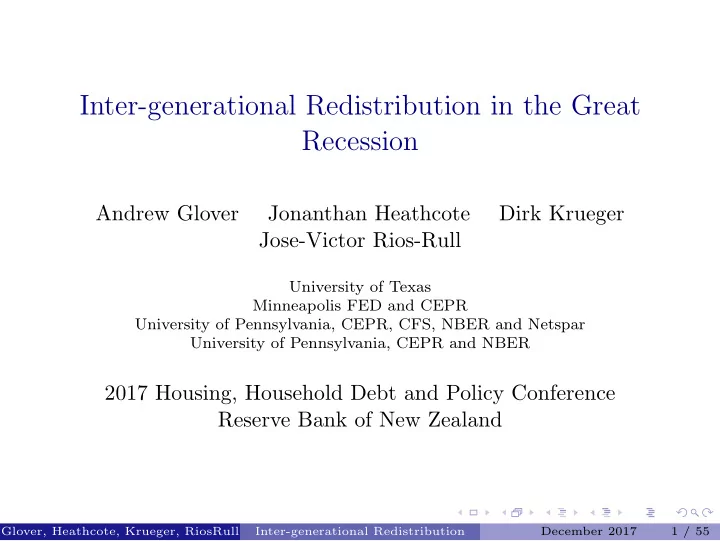
Inter-generational Redistribution in the Great Recession

Andrew Glover Jonanthan Heathcote Dirk Krueger Jose-Victor Rios-Rull

University of Texas Minneapolis FED and CEPR University of Pennsylvania, CEPR, CFS, NBER and Netspar University of Pennsylvania, CEPR and NBER

2017 Housing, Household Debt and Policy Conference Reserve Bank of New Zealand

Glover, Heathcote, Krueger, RiosRull Inter-generational Redistribution December 2017 1 / 55

SLIDE 2

Introduction

Salient features of the great recession:
Large fall in output and labor incomes.
Larger fall in asset prices (stocks, houses).
Research Question: What are the distributional consequences for

households at different stages of the life cycle?

Glover, Heathcote, Krueger, RiosRull Inter-generational Redistribution December 2017 2 / 55

SLIDE 3

Motivating Facts: Aggregate Data

2008 2009 2010 2011 2012 2013 2014 2015 Year

35
30
25
20
15
10
5

Percent Deviation from Trend Deviation of Real GDP pc, Asset Values, from 2% Trend Income Asset Values

Glover, Heathcote, Krueger, RiosRull Inter-generational Redistribution December 2017 3 / 55

SLIDE 4

Introduction

Paper relates directly to 3 themes stressed by Governor Spencer:
Housing is a key household asset.
(Mortgage) debt is an important part of household balance sheets.
Demographics is a key source of household heterogeneity

Glover, Heathcote, Krueger, RiosRull Inter-generational Redistribution December 2017 4 / 55

SLIDE 5

Introduction

Paper relates directly to 3 themes stressed by Governor Spencer:
Housing is a key household asset.
(Mortgage) debt is an important part of household balance sheets.
Demographics is a key source of household heterogeneity
Confessions [mainly to Chris]
I will do General Equilibrium with aggregate risk (so model is

DSGE, sort of).

My people have Euler equations
Limited heterogeneity within generations, but at least full life cycle

Glover, Heathcote, Krueger, RiosRull Inter-generational Redistribution December 2017 4 / 55

SLIDE 6

Introduction

Paper relates directly to 3 themes stressed by Governor Spencer:
Housing is a key household asset.
(Mortgage) debt is an important part of household balance sheets.
Demographics is a key source of household heterogeneity
Confessions [mainly to Chris]
I will do General Equilibrium with aggregate risk (so model is

DSGE, sort of).

My people have Euler equations
Limited heterogeneity within generations, but at least full life cycle
...so hopefully I am at least a bit Galilean
rather than look like poor old Ptolemy (who proposed an empirically

testable theory that was the leading paradigm for some 1300 years).

Glover, Heathcote, Krueger, RiosRull Inter-generational Redistribution December 2017 4 / 55

SLIDE 7

Motivating Facts

Why focus on age dimension?
Labor income and wealth vary substantially by age.
Portfolio composition (risky versus riskless assets) varies

substantially by age.

Labor income losses in great recession vary substantially by age.
(1) - (3) =

⇒ Wealth and welfare losses vary substantially by age.

Glover, Heathcote, Krueger, RiosRull Inter-generational Redistribution December 2017 5 / 55

SLIDE 8

Motivating Facts: Income and Wealth Over Life Cycle

Figure: Labor Income and Net Worth by Age, SCF 2007 ($1,000)

40.00 60.00 80.00 100.00 120.00 400.00 600.00 800.00 1000.00 1200.00 0.00 20.00 0.00 200.00 20-29 30-39 40-49 50-59 60-69 70 or more Age Group Net Worth (left axis) Labor Income (right axis)

Details of the Data Glover, Heathcote, Krueger, RiosRull Inter-generational Redistribution December 2017 6 / 55

SLIDE 9

Motivating Facts: Portfolio Shares by Age from 2007 SCF (in %)

(1) (2) (3) (4) (5) (6) (7) (8) (9) (10) Age Stk Res. Non Non Risky Bond Car Oth. Debt Safe Head RE bus. RE NW +CD NW All 30.3 47.0 12.9 3.8 94.0 17.0 3.5 4.2

18.6

6.0 20-29 13.2 77.7 43.3 1.3 135.5 13.7 15.3 4.5

68.9
35.5

30-39 26.3 96.5 12.7 5.0 140.4 13.8 9.7 4.2

68.2
40.4

40-49 30.4 57.6 12.6 3.8 104.4 15.2 4.4 4.5

28.5
4.4

50-59 32.7 42.4 13.5 3.7 92.4 17.0 2.8 4.0

16.1

7.7 60-69 32.2 35.6 13.4 4.1 85.3 17.5 2.4 4.7

9.9

14.7 70+ 27.1 39.8 9.0 3.3 79.2 19.3 1.8 3.7

3.9

20.8

Risky Net Worth (5) is equal to sum of columns (1)+(2)+(3)+(4). Safe Net Worth (10) is sum of columns (6)+(7)+(8)+(9). Total Net Worth is sum of (5)+(10)

Glover, Heathcote, Krueger, RiosRull Inter-generational Redistribution December 2017 7 / 55

SLIDE 10

Motivating Facts: Capital Losses by Age Group

Infl. adj. capital losses from 2007:2 to 2009:1-2013:4 ($1,000, 2007)

Age of Stocks Res. Nonc. Nonres. Total (%)net (%) Total/ Head RA bus. prop. worth inc. 2009Q1 All 30.6 64.4 15.1 6.5 116.5 21.0 139.6 154.5 20-29 1.9 14.8 7.1 0.3 24.0 31.1 61.9 24.5 30-39 9.5 47.5 5.4 3.0 65.4 32.8 93.7 73.0 40-49 25.7 66.1 12.3 5.4 109.6 23.5 117.3 139.8 50-59 49.1 86.4 23.6 9.4 168.5 20.4 142.8 232.3 60-69 61.5 92.4 29.8 13.3 197.0 18.7 180.6 278.9 70+ 35.9 71.4 13.8 7.4 128.5 17.6 223.2 173.9

Capital losses concentrated among older households

Glover, Heathcote, Krueger, RiosRull Inter-generational Redistribution December 2017 8 / 55

SLIDE 11

Motivating Facts: Change in Labor Income 2007 to 2010, Relative to Trend, CPS

(%) pc earnings

9.8

20-29

14.3

30-39

12.6

40-49

10.3

50-59

11.1

60-69

6.0

70+

1.4
Current earnings losses concentrated among younger households

Glover, Heathcote, Krueger, RiosRull Inter-generational Redistribution December 2017 9 / 55

SLIDE 12

Motivating Facts

Why focus on age dimension?
Labor income and wealth vary substantially by age.
Portfolio composition (risky versus riskless assets) varies

substantially by age.

Labor income losses in great recession vary substantially by age.
(1) - (3) =

⇒ Wealth and welfare losses vary substantially by age.

Glover, Heathcote, Krueger, RiosRull Inter-generational Redistribution December 2017 10 / 55

SLIDE 13

The Plan for Remainder of Talk

The Approach
Construct and compute a quantitative OLG model with aggregate

risk.

Calibrate it to life cycle facts from 2007 SCF.
Engineer a great recession.
Questions:
Can model generate magnitude of asset price declines as observed

in the data?

Can the model generate realistic age profile of asset portfolios?
How are wealth and welfare losses from great recession distributed

across different age cohorts?

Glover, Heathcote, Krueger, RiosRull Inter-generational Redistribution December 2017 11 / 55

SLIDE 14

An OLG Model with Aggregate Risk

Labor income and asset prices driven by aggregate shock

z ∈ Z = {zn, zr, zd} .

z follows Markov process with transition matrix Γz,z′.
Technology

Y (z) = zKθL1−θ = z

Supply of fixed factor (land, capital) normalized to K = 1. Labor

income (wages) equals w(z) = (1 − θ)z. Capital income equals θz.

Households live for I periods. Supply one unit of time, relative

labor efficiency (income) {εi(z)}I

i=1. Normalize i εi(z) = L = 1.

Time discount factors {βi}I

i=1 vary with age. Utility function

u(c) = c1−σ−1

1−σ . Wealth distribution A = {Ai}I i=1. No bequests.

Market Structure: Ownership shares of K traded at price p(z, A).

Exogenous net supply B of corporate bonds, price q(z, A).

Details of the Model Glover, Heathcote, Krueger, RiosRull Inter-generational Redistribution December 2017 12 / 55

SLIDE 15

Calibration Strategy

Model period 10 years. Agents enter at age 20, live for 6 periods.
Aggregate endowment process z ∈ Z = {zn, zr, zd} , Γz,z′ derived

directly from aggregate time series data. In Great Recession (zr)

utput falls 9.84%.
Life cycle profiles {βi, εi(z)} chosen so that model with z = zn

matches life cycle earnings and net worth profiles from 2007 SCF.

Choose (θ = 30%, B = 0.07) s.t. model matches 2007 SCF

aggregate wealth to earnings ratio (7.88), share of risky assets (91.8%).

Choose σ = 4.24 s.t. model ξ lines up with Great Recession

ξ = ∆W/∆z = 26.8%/9.84% = 2.7. Why need low IES 1/σ?

Glover, Heathcote, Krueger, RiosRull Inter-generational Redistribution December 2017 13 / 55

SLIDE 16

Calibration: Productivity Process

States z ∈ Z = {zn, zr, zd}. Normal times zn = 1, Great Recession

zr < 1, Great Depression zd < zr.

Set zr s.t. transition from zn to zr involves output decline of 9.84%

(average 2009-2013 deviation from 2% growth trend).

Set zd s.t. output in zd is 28.9% below zn, (average 1932-1936

deviation from trend).

Transition matrix Γ
Impose (perhaps arbitrary) restrictions Γn,d = Γr,r = Γd,r = 0.

Note: makes markets sequentially complete with two assets.

Choose Γn,r, Γr,d such that unconditional probability of Great

Recession is 13.7% and Great Depression is 2.84% (as estimated from Maddison data, 1800-2010.)

z =   1.0000 0.9016 0.7109   , Γz,z′ =     z 0.835 0.165 0.000 0.793 0.000 0.207 1.000 0.000 0.000

z′

    

Glover, Heathcote, Krueger, RiosRull Inter-generational Redistribution December 2017 14 / 55

SLIDE 17

Calibration: Earnings Losses in Great Recession

Estimate age-specific earnings declines (relative to aggregate

trend) from 2007 to 2010 using CPS data to obtain {εi(zr)}I

i=1.

(%) 20-29

14.3

30-39

12.6

40-49

10.3

50-59

11.1

60-69

6.0

70+

1.4

Average

9.8

Glover, Heathcote, Krueger, RiosRull Inter-generational Redistribution December 2017 15 / 55

SLIDE 18

Results: Asset Price Decline

1

1 2 3 4 5 6 7

30
20
10

10 % Dev From Pre-Recession Value

Prices

Stock Bond Wealth

1

1 2 3 4 5 6 7 Decades After Recession 3 4 5 6 7 Percent, Annualized

Expected Returns

Stock Bond

Thought experiment: Following long period of normal times, Great

Recession for 10 years with ∆z = 9.8%, then recovery.

p falls by 29.2% (σ > 1 is key), price of bonds q barely moves.
Positive expected consumption growth (q should fall)
But: Increase in income risk =

⇒ precautionary savings up. Keeps q from falling, risk free rate from rising (as in actual Great Recession).

Standard Asset Pricing Statistics Glover, Heathcote, Krueger, RiosRull Inter-generational Redistribution December 2017 16 / 55

SLIDE 19

Results: Portfolio Shares: Models and Data

20-29 30-39 40-49 50-59 60-69

Age Group

0.2 0.4 0.6 0.8 1 1.2 1.4 1.6 1.8 2 2.2

Risky Savings / Total Savings

Data Model Pre-Recession Model Recession

Share of risky assets in portfolio declines strongly with age. Why?
Markets sequentially complete =

⇒ All households born prior to recession share recession consumption risk perfectly.

For same risk exposure, young require more leveraged portfolios.
Portfolio age profile flattens in model Great Recession: Fear of Great

Depression curbs appetite of young for risky assets in Great Recession.

Endogenous portfolio shares depend too strongly on age. Will consider

model with exogenous (factual) portfolios.

Glover, Heathcote, Krueger, RiosRull Inter-generational Redistribution December 2017 17 / 55

SLIDE 20

Results: Welfare Losses from the Great Recession

Welfare measured as percentage change in consumption (in all

future dates, states) under no-recession scenario needed to make households indifferent between current state being zn and zr. Age ∆ Welf. 20-29

1.07%

30-39

4.78%

40-49

5.69%

50-59

7.48%

60-69

9.61%

70+

10.00%

Wealth-Based Welfare Measure Glover, Heathcote, Krueger, RiosRull Inter-generational Redistribution December 2017 18 / 55

SLIDE 21

Exploring the Welfare Losses: Consumption

1 2 3 4 5

14.00%
12.00%
10.00%
8.00%
6.00%
4.00%
2.00%

0.00% 2.00% 4.00% 6.00% 20-29 30-39 40-49 50-50 60-69 70+

Decades After Recession Consumption, % Difference

Immediate age-specific consumption response to recession

symmetric (−10%) across generations alive prior to recession.

Newborns see smaller consumption drop (relative to no recession

(−7.0%) percent. Permanent consumption advantage in future.

Glover, Heathcote, Krueger, RiosRull Inter-generational Redistribution December 2017 19 / 55

SLIDE 22

Importance of Asset Pricing Channel?

Three welfare impacts from Great Recession in baseline model:

1 Reduced PDV of future labor earnings 2 Reduced value of asset portfolio on impact 3 Gains from future asset price recovery

Now: Partial equilibrium with constant q′s. Goal: isolate effect 3.
Counterfactual A: Hold wealth distribution constant at onset of
recession. Only effect 1.
Counterfactual B: Reduction in age-specific wealth implied by asset

price fall. Effects 1 and 2.

Age Benchmark A (Eff 1.) B (Eff. 1. & 2.) 20-29

1.07
6.53
6.53

30-39

4.78
7.19
14.03

40-49

5.69
6.90
17.40

50-59

7.48
6.55
16.33

60-69

9.61
3.38
11.27

70+

10.00
1.88
10.00

Glover, Heathcote, Krueger, RiosRull Inter-generational Redistribution December 2017 20 / 55

SLIDE 23

Exogenous Portfolios

20-29 30-39 40-49 50-59 60-69

Age Group

0.4 0.6 0.8 1 1.2 1.4 1.6 1.8 2 2.2 2.4

Risky Savings / Total Savings

Model Data

Now households are forced to hold empirical portfolios (from 2007

SCF). Still make consumption-savings decisions.

Key plus: more realistic capital losses in Great Recession
Key minus: Asset price movements do not reflect time-varying

appetite for taking on aggregate risk.

Glover, Heathcote, Krueger, RiosRull Inter-generational Redistribution December 2017 21 / 55

SLIDE 24

Exogenous Portfolios

Elasticity of Asset Prices to Output. Key: bond prices fall a lot

too (big increase in risk-free rate in recession). Asset Endog. Exog. Wealth 2.72 2.02 Stock 2.97 2.08 Bond

0.07

1.31

Welfare? More significant welfare losses of very young, very old.

Age Endog. Exog. 20-29

1.07%
2.39%

30-39

4.78%
2.91%

40-49

5.69%
2.54%

50-59

7.48%
7.30%

60-69

9.61%
13.73%

70+

10.00%
11.37%

Glover, Heathcote, Krueger, RiosRull Inter-generational Redistribution December 2017 22 / 55

SLIDE 25

Welfare Losses from Recession by Age: Symmetric Earnings Losses

Given asset pricing channel, why do the young actually lose?
Answer: because they are especially hard-hit by the Great

Recession in the labor market. Age Bench.

Sym. ∆ Earn.

20-29

1.07%

0.32% 30-39

4.78%
5.04%

40-49

5.69%
5.90%

50-59

7.48%
7.64%

60-69

9.61%
9.74%

70+

10.00%
10.09%

Glover, Heathcote, Krueger, RiosRull Inter-generational Redistribution December 2017 23 / 55

SLIDE 26

Implications for the Dynamics of the Wealth Distribution: Model vs. Data

Endog. Portfolios
Exog. Portfolios

Data: NW, SCF Age 2007 2010 2013 2007 2010 2010 2007 2010 2013 20-29 0.00 0.00 0.00 0.00 0.00 0.00 2.30 1.27 1.50 30-39 6.29 4.20 7.74 6.25 5.67 5.75 5.95 4.20 6.05 40-49 14.73 11.98 14.61 14.42 14.06 13.35 13.94 13.97 14.25 50-59 25.59 25.20 25.23 25.31 25.28 24.90 24.70 24.52 22.92 60-69 31.76 34.71 31.21 32.03 32.44 31.84 31.45 32.66 30.53 70+ 21.62 23.91 21.21 21.99 22.55 24.16 21.67 23.38 24.74

Wealth share of young cohort (30-39) declines in Great Recession,

then rebounds. Both in model and in data.

Wealth Share of retiring cohort (60-69) increases in Great

Recession, then returns to normal. Both in model and in data.

Glover, Heathcote, Krueger, RiosRull Inter-generational Redistribution December 2017 24 / 55

SLIDE 27

Level- or Growth Rate Shocks?

So far aggregate output z mean reverting, thus in a great recession
utput and asset prices are expected to recover.
Robustness to permanent shocks to z? See also Khan (2017). We

explored this in a 3-generation OLG model calibrated to the same income losses.

Three basic results
For given risk aversion, asset price decline comparable to model with

trend-stationary output if (and only if ) output growth over ten or twenty years is negatively correlated, as in U.S. data (corr ≈ −0.55).

Absolute welfare losses from the great recession significantly larger

in the stochastic growth economy for all (but oldest) generation.

Relative welfare losses of young vs. middle aged comparable in both

economies.

Glover, Heathcote, Krueger, RiosRull Inter-generational Redistribution December 2017 25 / 55

SLIDE 28

Incorporating (Limited) Intra-Cohort Heterogeneity

Assume the wealthy are passive investors.
Calibrate model to bottom 90% earnings, wealth life cycle profile.
Requires (on average) less patient individuals.
Overall: asset price mechanism less relevant to bottom 90%.

Economy Age Group Baseline Low Wealth 20-29

1.07%
5.12%

30-39

4.78%
6.76%

40-49

5.69%
7.23%

50-59

7.48%
8.20%

60-69

9.61%
9.57%

70+

10.00%
9.88%

Glover, Heathcote, Krueger, RiosRull Inter-generational Redistribution December 2017 26 / 55

SLIDE 29

Conclusion

We have explored asset price implications of large recessions. Can

rationalize large price drops of (only) risky assets with fear of Great Recession (and IES 1/σ < 1).

We have explored the portfolio implications of the model. It can

account for (too much of the) relatively risky portfolios of young and relatively safe portfolios of the old in the data.

We have explored the redistributive implications of such
recessions. Old lose a lot, young little. Might have gained if it

wasn’t for the dismal labor market.

Heterogeneity within young generation?
Winners not the ones that don’t much participate in financial

markets ....

Glover, Heathcote, Krueger, RiosRull Inter-generational Redistribution December 2017 27 / 55

SLIDE 30

Conclusion

We have explored asset price implications of large recessions. Can

rationalize large price drops of (only) risky assets with fear of Great Recession (and IES 1/σ < 1).

We have explored the portfolio implications of the model. It can

account for (too much of the) relatively risky portfolios of young and relatively safe portfolios of the old in the data.

We have explored the redistributive implications of such
recessions. Old lose a lot, young little. Might have gained if it

wasn’t for the dismal labor market.

Heterogeneity within young generation?
Winners not the ones that don’t much participate in financial

markets ....

... bud rather those who plan to have large wealth-to-income ratio

in their 50’s.

Glover, Heathcote, Krueger, RiosRull Inter-generational Redistribution December 2017 27 / 55

SLIDE 31

What Is This Useful For?

Policy implications?
By construction nothing can be done about the recession itself.
But: government can of course affect distribution of welfare losses
r gains.
E.g. by purchasing assets at distressed prices (TARP?) government

may have mitigated welfare losses of elderly at expense of welfare gains of young.

Same might be true for expansion of outstanding government debt.

Glover, Heathcote, Krueger, RiosRull Inter-generational Redistribution December 2017 28 / 55

SLIDE 32

THANK YOU FOR COMING AND LISTENING

Glover, Heathcote, Krueger, RiosRull Inter-generational Redistribution December 2017 29 / 55

SLIDE 33

Discussion of the Assumptions I: Housing

Can re-interpret the model as explicit model of housing. Assume:
Fixed supply 1 of perfectly divisible houses. Competitive rental

markets.

Cobb Douglas utility over non-durables, housing services (cνs1−ν)

1−σ

Households can freely invest in three assets: bonds, stocks, houses.
Results: rents are proportional to dividends, housing prices

proportional to stock prices.

Thus model with housing has exactly the same asset pricing and

welfare implications as our model without explicit housing.

Glover, Heathcote, Krueger, RiosRull Inter-generational Redistribution December 2017 30 / 55

SLIDE 34

Discussion of the Assumptions II: Unemployment

In recession labor incomes fall because real wages w(z) = (1 − θ)z

fall, whereas hours worked L = 1 remain constant.

Could equivalently assume that labor income in recession falls due

to reduction in hours worked L(z): Y (z) = L(z)1−θ

As long as L(zr)/L(zn) = (zr/zn)

1 1−θ model with TFP shocks z

and model with aggregate shocks to hours worked L(z) (or aggregate shocks to unemployment) are isomorphic.

Glover, Heathcote, Krueger, RiosRull Inter-generational Redistribution December 2017 31 / 55

SLIDE 35

Calibration: Model with Exogenous Portfolios

Alternative version of the model in which savings is a choice, but

in which the portfolio shares are exogenous.

New parameters: age-varying portfolio shares {λi(z)}I

i=1.

Set equal to age-specific shares of risky assets from SCF:

Age λi(%) 20-29 135 30-39 140 40-49 104 50-59 92 60-69 85 70+ 79 Aggr. 94

Glover, Heathcote, Krueger, RiosRull Inter-generational Redistribution December 2017 32 / 55

SLIDE 36

Results

Asset Prices in a Great Recession
Portfolio Choices
Welfare Results
Quantifying the Asset Price Channel
Exploring the Sensitivity of Results
Exogenous (Data Implied) Portfolios
The Importance of Asymmetric Earnings Declines
Intracohort Heterogeneity

Glover, Heathcote, Krueger, RiosRull Inter-generational Redistribution December 2017 33 / 55

SLIDE 37

Motivating Facts: Income and Wealth Over the Life Cycle (2007 SCF, $1,000)

Total Labor Asset Assets Debts Net Worth Age Income Income Income All 83.43 70.07 13.36 659.00 103.34 555.66 20-29 38.83 39.68

0.85

130.66 53.30 77.36 30-39 69.83 68.68 1.15 335.87 136.12 199.75 40-49 93.40 84.97 8.43 598.21 132.62 465.59 50-59 117.97 99.56 18.41 959.77 133.24 826.53 60-69 109.06 76.15 32.90 1156.96 104.10 1052.86 70+ 57.56 34.46 23.11 756.76 28.48 728.28

Back to Plot Glover, Heathcote, Krueger, RiosRull Inter-generational Redistribution December 2017 34 / 55

SLIDE 38

Key Channel

The young have lots of future labor income, few financial assets.
Hurt by lower current wages, might benefit from lower asset prices.
Welfare consequences of downturn depend on:
Size of labor income asset price decline
Its persistence
Behavioral response of households (consumption-savings and

portfolio allocation choices).

Thus want labor income, asset prices and household choices be

endogenously determined in quantitative life cycle model.

Glover, Heathcote, Krueger, RiosRull Inter-generational Redistribution December 2017 35 / 55

SLIDE 39

The Model: Market Structure

Exogenous net supply B of corporate bonds. Unit supply of shares.
Aggregate state of the economy (z, A), where A = (A1, . . . , AI)

denotes the beginning of period wealth distribution across age cohorts.

Stock price p(z, A), bond price q(z, A).
Stocks pay dividends d(z, A) = θz − [1 − q(z, A)] B
Aggregate (start of period) wealth:

W(z, A) = p(z, A) + d(z, A) + B

Glover, Heathcote, Krueger, RiosRull Inter-generational Redistribution December 2017 36 / 55

SLIDE 40

Recursive Problem of the Household

State space (i, a, z, A), where a is the individual share of total

wealth W(z, A) held by the household. vi(a, z, A) = max

c≥0,y,λ,a′

u(c) + βi+1
z′∈Z

Γz,z′vi+1(a′, z′, A′)

c + y

= εi(z)w(z) + W(z, A)a a′W(z′, A′) =

λp(z′, A′) + d(z′, A′)

p(z, A) + (1 − λ) 1 q(z, A)

y

A′ = G(z, A, z′)

Policy functions ci(a, z, A), yi(a, z, A), λi(a, z, A) and a′

i(a, z, A, z′).

Glover, Heathcote, Krueger, RiosRull Inter-generational Redistribution December 2017 37 / 55

SLIDE 41

Equilibrium: Markets, Prices and Aggregation

Labor market: wages w(z) = (1 − θ)z and I

i=1 εi(z) = L = 1.

Financial Markets: Share prices p(z, S) and bond prices q(z, A)

I

i=1

yi(Ai, z, A)λi(Ai, z, A) = p(z, A)

I

i=1

yi(Ai, z, A) [1 − λi(Ai, z, A)] = q(z, A)B

Law of Motion: A′

1 = 0 and A′ i+1 = Gi+1(z, A, z′) = a′ i(Ai, z, A, z′).

Back to Model Glover, Heathcote, Krueger, RiosRull Inter-generational Redistribution December 2017 38 / 55

SLIDE 42

Calibration: Productivity Process

States z ∈ Z = {zn, zr, zd}. Normal times zn = 1, Great Recession

zr < 1, Great Depression zd < zr.

Set zr s.t. transition from zn to zr involves output decline of 9.84%

(average 2009-2013 deviation from 2% growth trend).

Set zd s. t. output in zd is 28.9% below zn, (average 1932-1936

deviation from trend).

Transition matrix Γ
Impose (perhaps arbitrary) restrictions Γn,d = Γr,r = Γd,r = 0.

Note: makes markets sequentially complete with two assets.

Choose Γn,r, Γr,d such that unconditional probability of Great

Recession is 13.7% and Great Depression is 2.84% (as estimated from Maddison data, 1800-2010.)

z =   1.0000 0.9016 0.7109   , Γz,z′ =     z 0.835 0.165 0.000 0.793 0.000 0.207 1.000 0.000 0.000

z′

    

Back to Calibration Glover, Heathcote, Krueger, RiosRull Inter-generational Redistribution December 2017 39 / 55

SLIDE 43

Developing Intuition: A Three Period Model

Key assumptions:
Households only productive when young: ε1 = 1, ε2 = ε3 = 0.
Households derive no utility from consumption when young. By

construction young save everything.

Only stocks are traded: B = 0.
Aggregate shock can only take two values: Z = {zr, zn}.
State (z, A) where A = A3 is share of assets held by old. Share of

wealth held by middle-aged is 1 − A.

Only middle-aged make meaningful decision: how many of their

shares to sell.

Note: wealth distribution irrelevant in Rep. Agent model or 2

period OLG model.

Glover, Heathcote, Krueger, RiosRull Inter-generational Redistribution December 2017 40 / 55

SLIDE 44

Developing Intuition: A Three Period Model

Measure of asset price collapse:

ξ(A) = log(p(zr, A)/p(zn, A)) log(zr/zn) Note: in RA economy with CRRA = σ, iid z shocks: ξRA = σ.

Choice of middle-aged: purchase shares A′ = G(z, A), at p(z, A)
Consumption when middle aged and old:

cm(z, A) = (1 − A) (p(z, A) + θz) − G(z, A)p(z, A) co(z, A; z′, A′) = G(z, A)p(z′, A′)

Euler equation

u′ [(1 − A) (p(z, A) + θz) − G(z, A)p(z, A)] = β

z′

Γz,z′ [p(z′, A′) + θz′] p(z, A) u′ G(z, A)p(z′, A′)

Second equation: young’s labor income equals their share purchase

[1 − G(z, A)]p(z, A) = (1 − θ)z

Glover, Heathcote, Krueger, RiosRull Inter-generational Redistribution December 2017 41 / 55

SLIDE 45

Developing Intuition: A Three Period Model

Solution is pair of functional equations in the unknown functions

p(z, A), G(z, A).

Consumption, welfare can be calculated from p(z, A), G(z, A).
Note: for log-utility complete analytical characterization of RCE:
Asset prices are proportional to output z, that is ξ = 1.
Wealth distribution (1 − A, A) does not respond to shock z.
Consumption of all generations move one for one with z.
If z is iid, then young are exactly indifferent between being born

into a Great Recession and being born into normal times.

Asset Price Decline Relative to Output

0.2 0.4 0.6 0.8 1 Wealth Share of Old 0.5 1 1.5 2 2.5 3 3.5 ξ Relative Asset Price Decline

sigma=0.4 sigma=1 sigma=4.24 sigma=8

The more households dislike consumption fluctuations (the higher

σ) the larger is the fall in p relative to z in the recession.

When IES = 1/σ < 1 a larger wealth share of the middle-aged

(smaller A) translates into greater asset price collapse ξ(A).

Glover, Heathcote, Krueger, RiosRull Inter-generational Redistribution December 2017 43 / 55

SLIDE 47

Welfare Consequences of Recessions for the Young

0.2 0.4 0.6 0.8 1 Wealth Share of Old

5

5 10 15 20 25 30 CEV Welfare Gain from Recession, Young

sigma=0.4 sigma=1 sigma=4.24 sigma=8 Zero Line

Welfare measured as % consumption equivalent variation (positive

numbers indicate welfare gains from recession).

Welfare consequences mirror the elasticity of asset prices to output.

Young can easily win from Great Recession. But in the simple model:

Young do not value consumption in Great Recession.
Young not disproportionally affected by labor income declines.
Middle-aged (and old) only have access to risky assets.

Glover, Heathcote, Krueger, RiosRull Inter-generational Redistribution December 2017 44 / 55

SLIDE 48

Logarithmic Utility (σ = 1)

Proposition

Let σ = 1 and εi(z) = εi ∀z. Then there exists a recursive competitive equilibrium such that

The distribution of wealth A = ¯

A = ( ¯ A1, . . . , ¯ AI) is constant over time: ∀z, z′, i = 1, ..., I − 1 Gi+1(z, ¯ A, z′) = a′

i(z, ¯

A, z′, ¯ Ai) = ¯ Ai+1 G1(z, ¯ A, z′) = ∀z, z′

Aggregate wealth is proportional to the aggregate shock: ∀z

p(z, ¯ A) + q(z, ¯ A)B = zΨ

Asset Portfolios are identical across age groups:

λi(z, ¯ A, ¯ Ai) = λ(z) = p(z) zΨ ∀z, ∀i = 1, ..., I − 1.

Consumption and savings at each age are given by:

ci(z, ¯ A, ¯ Ai) = z

(1 − θ)εi + θ ¯

Ai + ¯ Ai − ¯ Ai+1

Ψ
,

yi(z, ¯ A, ¯ Ai) = z ¯ Ai+1Ψ ∀z, ∀i = 1, ..., I − 1. back Glover, Heathcote, Krueger, RiosRull Inter-generational Redistribution December 2017 45 / 55

SLIDE 49

Logarithmic Utility (σ = 1)

Proposition

Let σ = 1 and εi(z) = εi ∀z. Then there exists a recursive competitive equilibrium with the following properties:

Stock and bond prices are given by

p(z, ¯ A) = p(z) = zΨ − B z R

z′∈Z

Γz,z′ 1 z′ q(z, ¯ A) = q(z) = z R

z′∈Z

Γz,z′ 1 z′ ∀z. where R = (Ψ + θ)/Ψ.

The equity premium is given by

R

z

Πz z             

z′∈Z

Γz,z′ z′ −

z′∈Z

Γz,z′ 1

z′

−1 1 −

B RΨ

z′∈Z

Γz,z′ 1

z′

             back Glover, Heathcote, Krueger, RiosRull Inter-generational Redistribution December 2017 46 / 55

SLIDE 50

Logarithmic Utility (σ = 1)

Proposition

If z is iid then for all z ∈ Z p(z) = z  Ψ − B R

z′∈Z

Πz′ 1 z′   q(z) = z   1 R

z′∈Z

Πz′ 1 z′   and the average equity premium is given by R

z

Πz z

z

Πzz − 1

1 −

B RΨ

z

Πz z

Proposition

In the limit as Γz,z → 1 ∀z (perfectly persistent shocks), q(z) → R−1 and p(z) → zΨ − BR−1. back Glover, Heathcote, Krueger, RiosRull Inter-generational Redistribution December 2017 47 / 55

SLIDE 51

Wealth-Based Welfare Measures

Wealth-based welfare measure invariant to remaining lifetime

horizon.

How much must wealth be reduced in the no-recession state for

households to be indifferent between life with or without the recession in the current period?

Normalize wealth measure by pc consumption in normal times.

back

Age Bench.

Sym. ∆ Earn.

Exog. 20-29

1.98%

0.60%

3.90%

30-39

11.20%
11.87%
6.30%

40-49

15.79%
16.38%
6.83%

50-59

22.83%
23.31%
20.39%

60-69

25.90%
26.24%
35.77%

70+

14.95%
15.08%
19.11%

Glover, Heathcote, Krueger, RiosRull Inter-generational Redistribution December 2017 48 / 55

SLIDE 52

Standard Asset Pricing Statistics

Return Stats: Benchmark Model Asset Average

Std. Dev.
Corr. w/ Stock

Stock 4.50% 31.2% 1.00 Bond 4.09% 25.3% 0.79 Return Stats: Model w/o Great Depr. Asset Average

Std. Dev.
Corr. w/ Stock

Stock 4.41% 16.6% 1.00 Bond 3.68% 1.2%

0.07

Return Stats: Data Asset Average

Std. Dev.
Corr. w/ Stock

Stock 6.62% 36.4% 1.00 Bond 2.29% 30.4% 0.01

back Glover, Heathcote, Krueger, RiosRull Inter-generational Redistribution December 2017 49 / 55

SLIDE 53

Implications for the Dynamics of the Wealth Distribution: Model vs. Data

Model End. Portf. Model Exog. Portf. Data Age PreR Rec. Reco PreR Rec. Reco 2007 2010 2013 20-29 0.0 0.0 0.0 0.0 0.0 0.0 2.3 1.3 1.5 30-39 2.6

1.4

6.0 4.9 3.9 4.5 6.0 4.2 6.1 40-49 9.9 4.6 12.0 13.6 13.0 12.5 13.9 14.0 14.3 50-59 24.9 24.1 23.4 25.2 25.2 24.8 24.7 24.5 22.9 60-69 36.9 42.6 32.8 33.0 33.7 32.7 31.5 32.7 30.5 70+ 25.6 30.1 25.8 23.3 24.2 25.6 21.7 23.4 24.7

Glover, Heathcote, Krueger, RiosRull Inter-generational Redistribution December 2017 50 / 55

SLIDE 54

Level- or Growth Rate Shocks?

So far aggregate output z mean reverting, thus in a great recession
utput and asset prices are expected to recover.
Robustness to permanent shocks to z? Consider 3-period model

but assume that g′ = z′/z follows Markov process with Γg,g′.

Calibrate s.t. output falls 9.83% in recession.
Three basic results
For given risk aversion, ξ comparable to model with

trend-stationary output if (and only if ) output. growth over ten or twenty years negatively correlated, as in U.S. data (corr ≈ −0.55).

Absolute welfare losses from the great recession significantly larger

in the stochastic growth economy (for all but oldest generation).

Relative welfare losses by age are comparable in both economies.

Glover, Heathcote, Krueger, RiosRull Inter-generational Redistribution December 2017 51 / 55

SLIDE 55

Asset Prices: Two Economies

0.1 0.2 0.3 0.4 0.5 0.6 0.7 0.8 0.9 Wealth Share of Old 0.5 1 1.5 2 2.5 3 3.5 4 ξ Relative Asset Price Decline

sigma=1, Growth Rates sigma=1, Levels sigma=4.24, Growth Rates sigma=4.24, Levels sigma=8.0, Growth Rates sigma=8.0, Levels Glover, Heathcote, Krueger, RiosRull Inter-generational Redistribution December 2017 52 / 55

SLIDE 56

Relative Welfare Losses by Age: Two Economies

Economy Age Group Shocks to z Shocks to z′/z Old (absolute) −12.3% −11.4% Middle (absolute) −3.7% −6.0% Young (absolute) 2.9% −5.0% Middle rel.to Old 8.6% 5.4% Young rel. to Old 15.2% 6.4%

Glover, Heathcote, Krueger, RiosRull Inter-generational Redistribution December 2017 53 / 55

SLIDE 57

Incorporating (Limited) Intra-Cohort Heterogeneity

Are welfare losses of ”average household” within an age group

representative? Now consider limited intra-cohort heterogeneity.

Two types of households: a wealthy type and a low-wealth type.
Assume that wealthy type accounts for a fixed fraction κy of

aggregate labor earnings, passively holds a fixed fraction κa of aggregate debt, equity.

Thus the wealthy consume a fixed fraction (1 − θ)κy + κaθ of

aggregate output at each date.

Assets are priced by the low-wealth type, and prices fluctuate such

that this type always demands (1 − κa) shares and κaB bonds.

In essence: recalibration of a model with lower income- and wealth
households. Key difference: wealth-to-income ratio is lower among

asset pricers now.

Results fairly unchanged relative to baseline model, but asset price

channel somewhat less important.

Glover, Heathcote, Krueger, RiosRull Inter-generational Redistribution December 2017 54 / 55

SLIDE 58

Related Literature

OLG economies with aggregate risk:
Asset pricing: Labadie (1986), Huffman (1987), Constantinides,

Donaldson and Mehra (2002), Storesletten, Telmer and Yaron (2007), Kubler and Schmedders (2015)

Allocations: a) Business cycles: Rios-Rull (1994, 1996), Gomes,

Michaelides and Polkovnichenko (2010), b) Intergenerational risk sharing: Bohn (1998), Shiller (1999), Demange (2002), Smetters (2006), Krueger and Kubler (2006), Ball and Mankiw (2007), Miyazaki, Sato and Yamada (2009), Olovsson (2010).

Redistributional consequences by age of other aggregate shocks:
Inflation: Doepke and Schneider (2006a,b), Meh, Rios-Rull and

Terajima (2010).

Demographics: Demange and Laroque (1999), Rios-Rull (2001),

Abel (2003), Attanasio, Kitao and Violante (2007), Krueger and Ludwig (2007).

Consumption disasters: Barro (2006, 2009), Nakamura, Steinsson,

Barro and Ursua (2013), Gourio (2010).

Glover, Heathcote, Krueger, RiosRull Inter-generational Redistribution December 2017 55 / 55