InGrid 2.0 Study of poverty measurement on context-specific - PowerPoint PPT Presentation
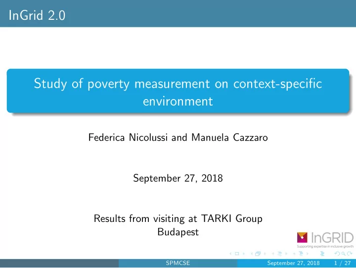
InGrid 2.0 Study of poverty measurement on context-specific environment Federica Nicolussi and Manuela Cazzaro September 27, 2018 Results from visiting at TARKI Group Budapest SPMCSE September 27, 2018 1 / 27 Overview Introduction 1
InGrid 2.0 Study of poverty measurement on context-specific environment Federica Nicolussi and Manuela Cazzaro September 27, 2018 Results from visiting at TARKI Group Budapest SPMCSE September 27, 2018 1 / 27
Overview Introduction 1 Models 2 Graphical model Multivariate Regression parametrization Application 3 Results Conclusions 4 Acknowledgement 5 References 6 SPMCSE September 27, 2018 2 / 27
Introduction Framework : q categorical (ordinal) variables Q = { X 1 , . . . , X q } collected in a contingency table. study of (in)dependence relationships among these variables. SPMCSE September 27, 2018 3 / 27
Introduction Framework : q categorical (ordinal) variables Q = { X 1 , . . . , X q } collected in a contingency table. study of (in)dependence relationships among these variables. Main goals : 1) to consider different kind of relationships ( marginal , conditional and context-specific independencies in the same model) 2) to represent these relationships through graphical model [Stratified chain graph model]. 3) to represent the variables in a multivariate regression system [Regression parameters]; SPMCSE September 27, 2018 3 / 27
Example of potential relationships among the variables (AIM 1) Let us consider 3 variables A , B and C , for instance A Gender (M,F); B University Position (Student, PhD and Post Doc, Academic staff and Tecnical and administrative staff); C Age ( ≤ 25, 25 ⊣ 40, > 40). SPMCSE September 27, 2018 4 / 27
Example of potential relationships among the variables (AIM 1) Let us consider 3 variables A , B and C , for instance A Gender (M,F); B University Position (Student, PhD and Post Doc, Academic staff and Tecnical and administrative staff); C Age ( ≤ 25, 25 ⊣ 40, > 40). MARGINAL INDEPENDENCE : A ⊥ C → GENDER ⊥ AGE SPMCSE September 27, 2018 4 / 27
Example of potential relationships among the variables (AIM 1) Let us consider 3 variables A , B and C , for instance A Gender (M,F); B University Position (Student, PhD and Post Doc, Academic staff and Tecnical and administrative staff); C Age ( ≤ 25, 25 ⊣ 40, > 40). MARGINAL INDEPENDENCE : A ⊥ C → GENDER ⊥ AGE CONDITIONAL INDEPENDENCE : A ⊥ B | C → GENDER ⊥ POSITION | AGE SPMCSE September 27, 2018 4 / 27
Example of potential relationships among the variables (AIM 1) Let us consider 3 variables A , B and C , for instance A Gender (M,F); B University Position (Student, PhD and Post Doc, Academic staff and Tecnical and administrative staff); C Age ( ≤ 25, 25 ⊣ 40, > 40). MARGINAL INDEPENDENCE : A ⊥ C → GENDER ⊥ AGE CONDITIONAL INDEPENDENCE : A ⊥ B | C → GENDER ⊥ POSITION | AGE CONTEXT-SPECIFIC INDEPENDENCE : A ⊥ B | C = c k → GENDER ⊥ POSITION | AGE = ( > 40) SPMCSE September 27, 2018 4 / 27
Graphical representation: (AIM 2) ⋆ These different kind of independencies can be highlighted with a representation taking advantage of the Graphical Model SPMCSE September 27, 2018 5 / 27
Graphical representation: (AIM 2) ⋆ These different kind of independencies can be highlighted with a representation taking advantage of the Graphical Model ⋆ The three kinds of independencies can be well represented by the so-called Stratified Chain Graph Model (SCGM) SPMCSE September 27, 2018 5 / 27
Stratified regression chain graph models A GRAPH is defined as a set of vertices (V) and edges (E). The edge can be undirected or directed (arrow). B B A C A A E C C B D SPMCSE September 27, 2018 6 / 27
Stratified regression chain graph models ⋆ Vertices act as variables ⋆ Any Missing Arc is a symptom of A C independence E B D SPMCSE September 27, 2018 7 / 27
Stratified regression chain graph models ⋆ Vertices act as variables ⋆ Any Missing Arc is a symptom of A C independence ⋆ Markov properties: missing undirected arc ( C − D ): E C ⊥ D | AB missing directed arc ( B → C ): C ⊥ B | A missing directed arcs B D ( A → E ) and ( B → E ): E ⊥ AB | CD SPMCSE September 27, 2018 7 / 27
Stratified regression chain graph models ⋆ Any Directed Arc links a covariate with a response variable A C ⋆ Any Undirected Arc describes symmetrical dependence (among a set of covariate or among a set of E dependent variables) B D SPMCSE September 27, 2018 8 / 27
Stratified regression chain graph models ⋆ Any Directed Arc links a covariate with a response variable A C ⋆ Any Undirected Arc describes symmetrical dependence (among a set of covariate or among a set of E dependent variables) ⋆ A,B: covariate; ⋆ C,D,E: dependent variables; B D SPMCSE September 27, 2018 8 / 27
Stratified regression chain graph models ⋆ Labelled arcs report the list of modality(ies) of variable(s) according to the context-specific independence A C C ⊥ D | AB = ( a 1 , ∗ ) AB=(a 1 , ∗ ) E B D SPMCSE September 27, 2018 9 / 27
Multivariate Regression parametrization (AIM 3) Given two sets of variables: the response variables ( C and D ) and the covariates ( A and B ), the multivariate regression models is: η ABC β C ∅ + β C A ( i A ) + β C B ( i B ) + β C ( i C | i A i B ) = AB ( i A i B ) C η ABD β D ∅ + β D A ( i A ) + β D B ( i B ) + β D ( i D | i A i B ) = AB ( i A i B ) D η ABCD β CD + β CD A ( i A ) + β CD B ( i B ) + β CD ( i CD | i A i B ) = AB ( i A i B ) CD ∅ η are log-linear parameters (contrasts of logarithms -of sum- of probabilities) that are defined on marginal tables (by respecting completeness and hierarchical properties), Bartolucci, Colombi and Forcina, 2007; the regression β parameters are a function of the η parameters. SPMCSE September 27, 2018 10 / 27
Model definition (constraints on regression parameters) From the missing arcs to the constraints on regression parameters MISSING UNDIRECTED ARC ( C − D ) : C ⊥ D | AB A C η ABCD ( i C i D | i A i B ) = 0 ∀ i A , i B , i C , i D CD E MISSING DIRECTED ARC ( B → C ) : B ⊥ C | A B D η ABC ( i C | i A i B ) = β C ∅ + β C A ( i A ) ∀ i A , i B , i C C SPMCSE September 27, 2018 11 / 27
Model definition (constraints on regression parameters) From the labelled arcs to the constraints on regression parameters LABELLED UNDIRECTED ARC ( C − D ) : C ⊥ D | AB = ( a 1 , ∗ ) A C A=(a 1 ) η ABCD ( i C i D | i ′ A i ′ B ) = 0 AB=(a 1 , ∗ ) ∀ i C , i D and i ′ A i ′ B =( a 1 , ∗ ) CD E LABELLED DIRECTED ARC ( B → C ) : B D B ⊥ C | A = a 1 ( i C | i ′ A ( i ′ η ABC A i B ) = β C ∅ + β C A ) ∀ i B , i C and i ′ A = a 1 C SPMCSE September 27, 2018 12 / 27
At glance Graph gives a system of independencies; The unconstrained parameters describe the dependence relationships; The system of independencies identifies the regression parameters constrained to zero; A model is estimated through the Likelihood Ratio test. SPMCSE September 27, 2018 13 / 27
Selection of the best fitting model Step 1 Exploratory phase where we test all SCRGMs with only one missed arc. We consider as reduced model the one with the missing arcs that have lead to a p-value greater than 0 . 01; Step 2 We start from the reduced model and we add one by one all arcs. We choose the HMM model with lowest AIC; Step 3 We proceed to a further simplification of the model by replacing the missing arcs with labelled arcs. We choose with lowest AIC among the ones with p-value greater or equal to 0 . 05. SPMCSE September 27, 2018 14 / 27
Data Set We consider the subjects from 26 European countries which the self-defined current economic status (variable PL031 in the survey) is (i) employee working full-time , (ii) employee working part-time , (iii) self-employed working full-time , (iv) self-employed working part-time , (v) unemployed , (vi) permanently disabled or/and unfit to work or (vii) fulfilling domestic tasks and care responsibilities . The survey covers 288132 individuals. SPMCSE September 27, 2018 15 / 27
Variables G Gender (1= male, 2= female); A Age, categorized in 4 values representing the quartiles (1= 16 ⊢ 36; 2= 36 ⊢ 46; 3= 46 ⊢ 55; 4= 55 ⊢ 81); W Status in employment (1= self-employed with employees, 2= self-employed without employees, 3= employee, 4= family worker, 5= unemployed) H General health (1= very good, 2= good, 3= fair, 4= bad, 5= very bad) P Poverty indicator (0= equivalised disposable income ≥ at risk of poverty threshold, 1= equivalised disposable income < at risk of poverty threshold) AIMS : How gender and age affect the working condition and the general perceived health; How these variables affect the poverty indicator. SPMCSE September 27, 2018 16 / 27
Some information We have 288132 observations. We collect the 5 variables in a contingency table of 400 cells where only 33 cells are null. The class of marginal sets is { ( G , A ); ( G , A , W ); ( G , A , H ); ( G , A , W , H ); ( G , A , W , H , P ) } SPMCSE September 27, 2018 17 / 27
Mosaic Plots Representation of the distribution of G and P in two conditional distributions. (left) evidence of dependence between G and P ; (right) evidence of independence between G and P . A, H, W = 4,1,5 A, H, W = 1,5,5 P P 0 1 0 1 deviance deviance residuals: residuals: 5.7 0.052 1 4.0 1 2.0 G G 0.000 0.0 2 −2.0 2 −3.9 −0.046 p−value = p−value = 8.8224e−16 0.93214 SPMCSE September 27, 2018 18 / 27
Recommend
More recommend
Explore More Topics
Stay informed with curated content and fresh updates.


