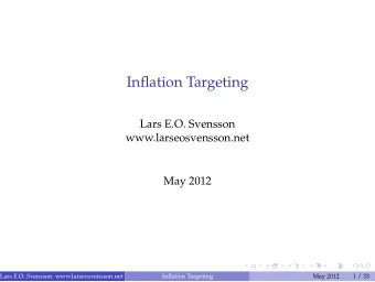
Inflation Targeting Lars E.O. Svensson larseosvensson.se May 2014 - PDF document

Inflation Targeting Lars E.O. Svensson larseosvensson.se May 2014 Lars E.O. Svensson larseosvensson.se () Inflation Targeting May 2014 1 / 33 Outline (in Friedman and Woodford, eds., Handbook of Monetary Economics, Volume 3b , chapt. 22, Elsevier, 2010) 1 Introduction: Inflation targeting An announced numerical inflation target 1 Forecast targeting, flexible inflation targeting: Choose policy rate 2 path so forecast of inflation and real economy “looks good” (stabilizes inflation around target and resource utilization around normal) A high degree of transparency and accountability 3 2 History and macroeconomic effects Starts 1990 in NZ, now about 25 countries Effects on inflation, inflation expectations, and output Success: Flexible, resilient, and robust monetary-policy regime Lars E.O. Svensson larseosvensson.se () Inflation Targeting May 2014 2 / 33

Outline 3 Theory Central role of projections Policy choice: Choice of interest-rate path, not policy function, in feasible set of projections Targeting rules Implementation of policy and equilibrium determination Uncertainty: State of the economy (additive), the transmission mechanism (model, multiplicative) Judgment Lars E.O. Svensson larseosvensson.se () Inflation Targeting May 2014 3 / 33 Outline 4 Practice Publishing a policy-rate path Case studies: The Riksbank and Norges Bank (Fed could now be added!) (Preconditions for emerging-market economics) 5 Future (Price-level targeting) (Inflation targeting and financial stability: Lessons from the financial crisis) 6 Conclusions Lars E.O. Svensson larseosvensson.se () Inflation Targeting May 2014 4 / 33

2 History and macroeconomic effects Inflation targeting starts 1990 in New Zealand Bundesbank inflation targeter in disguise? Now about 10 advanced and 15 emerging-market and developing countries Lars E.O. Svensson larseosvensson.se () Inflation Targeting May 2014 5 / 33 2 History: Approximate adoption dates Country Date Country Date New Zealand 1990 q1 Korea 2001 m1 Canada 1991 m2 Mexico 2001 m1 United Kingdom 1992 m10 Iceland 2001 m3 Sweden 1993 m1 Norway 2001 m3 Finland 1993 m2 Hungary 2001 m6 Australia 1993 m4 Peru 2002 m1 Spain 1995 m1 Philippines 2002 m1 Israel 1997 m6 Guatemala 2005 m1 Czech Republic 1997 m12 Slovakia 2005 m1 Poland 1998 m10 Indonesia 2005 m7 Brazil 1999 m6 Romania 2005 m8 Chile 1999 m9 Turkey 2006 m1 Colombia 1999 m9 Serbia 2006 m9 South Africa 2000 m2 Ghana 2007 m5 Thailand 2000 m5 U.S. 2012 m1 Lars E.O. Svensson larseosvensson.se () Inflation Targeting May 2014 6 / 33

2 History and macroeconomic effects Effects on inflation, inflation expectations, and output for advanced and emerging-market countries Success: Flexible, robust, and resilient monetary-policy regime Lars E.O. Svensson larseosvensson.se () Inflation Targeting May 2014 7 / 33 3 Theory Linear quadratic model (approximation around stochastic steady state) � � � X t � � C � X t + 1 = A + Bi t + ε t + 1 (1) Hx t + 1 | t x t 0 X t predetermined , x t forward-looking variables, i t (policy) instruments , x t + 1 | t ≡ E t x t + 1 , ε t i.i.d. zero-mean shocks x t determined by x t + 1 | t , X t , i t : Hx t + 1 | t = A 21 X t + A 22 x t + B 2 i t A − 1 x t = 22 ( Hx t + 1 | t − A 21 X t − B 2 i t ) X t + 1 determined by X t , x t , i t , ε t + 1 : X t + 1 = A 11 X t + A 12 x t + B 1 i t + C ε t + 1 Lars E.O. Svensson larseosvensson.se () Inflation Targeting May 2014 8 / 33

3 Theory Example: New Keynesian model (indexing to average inflation, π ≡ E [ π t ] ; credible inflation target, E [ π t ] = π ∗ ) ¯ π t − ¯ = δ ( π t + 1 | t − ¯ π ) + κ ( y t − ¯ y t ) + ξ t π = ρ u ξ t + ε ξ , t + 1 ξ t + 1 y t − ¯ y t = ( y t + 1 | t − ¯ y t + 1 | t ) − σ ( i t − π t + 1 | t − ¯ r t ) ¯ r t + 1 = ρ r ¯ r t + ε r , t + 1 ( ¯ y t + 1 | t − ¯ y t = σ ¯ r t ) r t ) � X t = ( 1, ξ t , ¯ y t ) � x t = ( π t , y t − ¯ i t = i t ( ε ξ t , ε rt ) � ε t = Lars E.O. Svensson larseosvensson.se () Inflation Targeting May 2014 9 / 33 3 Theory Y t target variables, typically Y t ≡ ( π t − π ∗ , y t − ¯ y t , ... ) � ⎡ ⎤ X t ⎣ ⎦ Y t = D x t (2) i t Intertemporal loss function ∞ δ τ L t + τ ( 0 < δ < 1 ) ∑ E t (3) τ = 0 Period loss L t ≡ Y � t Λ Y t (4) Λ weight matrix, typically Λ ≡ Diag ( 1, λ , ... ) L t = ( π t − π ∗ ) 2 + λ ( y t − ¯ y t ) 2 Lars E.O. Svensson larseosvensson.se () Inflation Targeting May 2014 10 / 33

3 Theory Optimization under commitment in a timeless perspective, solution: � x t � � � � F x � � � X t X t = F ≡ (5) i t Ξ t − 1 F i Ξ t − 1 � X t + 1 � � � � C � X t = M + ε t + 1 (6) Ξ t Ξ t − 1 0 � I 0 � � � � � X t X t ≡ ˜ Y t = D D (7) Ξ t − 1 Ξ t − 1 F Ξ t Lagrange multipliers for lower block of (1) Optimal instrument rule (optimal policy function), � � X t i t = F i (8) Ξ t − 1 Certainty equivalence: Matrices F and M depend on A , B , H , D , Λ , and δ , but not on C Lars E.O. Svensson larseosvensson.se () Inflation Targeting May 2014 11 / 33 3 Theory Standard theory of (optimal) monetary policy: Central bank commits to some (optimal) policy function F i Private sector combines policy function with model, solves for rational-expectations equilibrium Not in practice: Inflation-targeting central bank chooses and announces current policy rate, indicates or announces path of future policy rate, publishes forecast of inflation and the real economy Private sector responds to this information, and the actual equilibrium results Forecasts and projections of the policy rate, inflation, and the real economy take center stage How to model and understand? Lars E.O. Svensson larseosvensson.se () Inflation Targeting May 2014 12 / 33

3 Theory All inflation-targeting central banks not well described by this theory Theory is idealization (like consumption theory of actual consumer behavior) Theory of mature inflation targeting, potential best-practice inflation targeting Actual inflation targeting, w/ one innovation after the other, moving in this direction Some inflation-targeting central banks may be pretty close Lars E.O. Svensson larseosvensson.se () Inflation Targeting May 2014 13 / 33 3 Theory Some misunderstandings to be avoided: Two things that inflation targeting is not (cf. Orphanides) Not strict inflation targeting, not L t = ( π t − π ∗ ) 2 . In practice always flexible inflation targeting (but not necessarily transparent). Not simple policy rule, such that i t = α ( π t − π ∗ ) or i t − i t − 1 = α ( π t − π ∗ ) . Instead, inflation targeting implies that central banks respond to much more information, namely all information that affects the forecast of inflation and the real economy (resource utilization) Lars E.O. Svensson larseosvensson.se () Inflation Targeting May 2014 14 / 33

3.2 Projection model; feasible set of projections u t ≡ { u t + τ , t } ∞ τ = 0 projection (conditional mean forecast) in period t Projection model for the projections ( X t , x t , i t , Y t ) in period t ( ε t + τ , t = 0 for τ ≥ 1) � X t + τ + 1, t � � X t + τ , t � = A + Bi t + τ , t (9) Hx t + τ + 1, t x t + τ , t ⎡ ⎤ X t + τ , t ⎣ ⎦ Y t + τ , t = D x t + τ , t (10) i t + τ , t X t , t = X t | t (11) X t | t estimate of predetermined variables in period t (allows for imperfectly observed state of the economy) T ( X t | t ) feasible set of projections for given X t | t , the set of projections ( X t , x t , i t , Y t ) that satisfy (9)-(11) Lars E.O. Svensson larseosvensson.se () Inflation Targeting May 2014 15 / 33 3.3 Optimal policy choice Policy problem in t : Determine optimal projection ( ˆ ı t , ˆ X t , ˆ x t , ˆ Y t ) , projection that minimizes intertemporal forecast loss function, ∞ L ( Y t ) = δ τ L t + τ , t ( 0 < δ ≤ 1 ) , ∑ (12) τ = 0 subject to ( X t , x t , i t , Y t ) ∈ T ( X t | t ) Period forecast loss L t + τ , t ≡ Y t + τ , t � Λ Y t + τ , t (13) Optimization under commitment in timeless perspective, modified loss function (Svensson-Woodford 05) � � L ( Y t ) + 1 δ Ξ � s.t. ( X t , x t , i t , Y t ) ∈ T ( X t | t ) t − 1 H ( x t , t − x t , t − 1 ) min i t , Y t (14) Lars E.O. Svensson larseosvensson.se () Inflation Targeting May 2014 16 / 33

3.3 Optimal policy choice Alternative implementation of timeless perspective (Giannoni-Woodford 02, Svensson-Woodford 05): Restriction instead of modified loss function � X t | t � x t , t = F x (15) Ξ t − 1 T ( X t | t , Ξ t − 1 ) , the restricted feasible set of projections , the subset of the feasible set of projections T ( X t | t ) that satisfy (15) for given X t | t and Ξ t − 1 Optimal policy projection is also the solution to the problem i t , Y t L ( Y t ) subject to ( X t , x t , i t , Y t ) ∈ T ( X t | t , Ξ t − 1 ) min (16) Lars E.O. Svensson larseosvensson.se () Inflation Targeting May 2014 17 / 33 3.4 The forecast Taylor curve ∞ ∞ δ τ ( π t + τ , t − π ∗ ) 2 + λ L ( Y t ) = δ τ ( y t + τ , t − ¯ y t + τ , t ) 2 ∑ ∑ (17) τ = 0 τ = 0 Sums of discounted squared inflation and output gaps (forecasts) Lars E.O. Svensson larseosvensson.se () Inflation Targeting May 2014 18 / 33