Inference and Optimalities in Estimation of Gaussian Graphical Model - PowerPoint PPT Presentation
Inference and Optimalities in Estimation of Gaussian Graphical Model Harrison H. Zhou Department of Statistics Yale University Jointly with Zhao Ren, Tingni Sun and Cun-Hui Zhang 1 Outline Introduction Main Results Asymptotic
Inference and Optimalities in Estimation of Gaussian Graphical Model Harrison H. Zhou Department of Statistics Yale University Jointly with Zhao Ren, Tingni Sun and Cun-Hui Zhang 1
Outline • Introduction • Main Results – Asymptotic Efficiency – Rate-optimal Estimation of Each Entry • Applications – Adaptive Support Recovery – Estimation Under the Spectral Norm – Latent Variable Graphical Model • Summary 2
Introduction Gaussian Graphical Model: Let G = ( V, E ) be a graph. V = { Z 1 , . . . , Z p } is the vertex set and E is the edge set representing conditional dependence relations between the variables. Consider Z = ( Z 1 , Z 2 , . . . , Z p ) T ∼ N 0 , Ω − 1 ) ( , where Ω = ( ω ij ) 1 ≤ i,j ≤ p . Question: Are Z i and Z j conditionally independent given Z { i,j } c ? 3
Conditional Independence Property: The conditional distribution of Z A given Z A c is − Ω − 1 A,A Ω A,A c Z A c , Ω − 1 ( ) Z A | Z A c = N , A,A where A ⊂ { 1 , 2 , . . . , p } . Example: Let A = { 1 , 2 } . The precision matrix of ( Z 1 , Z 2 ) T given Z { 1 , 2 } c is ω 11 ω 12 . Ω A,A = ω 21 ω 22 Hence Z 1 ⊥ Z 2 | Z { 1 , 2 } c ⇐ ⇒ ω 12 = 0. 4
An Old Example Whittaker (1990): Examination marks of 88 students in 5 different mathematical subjects, Analysis, Statistics, Mechanics, Vectors, Algebra. Vectors Analysis ❢ ❢ ◗◗◗◗◗◗◗◗◗ ✑ ✑ ✑ ✑ ✑ ✑ Algebra ✑ ✑ ✑ ◗ ✑ ❢ ✑ ◗ ✑✑✑✑✑✑✑✑✑ ◗ ◗ ◗ ◗ ◗ ◗ ◗ ◗ ◗ ❢ ❢ Mechanics Statistics Remark { Analysis, Stats } ⊥ { Mech, Vectors } | Algebra. 5
What to do when p is very large? 6
Assumptions Consider a class of sparse precision matrices G 0 ( M, k n,p ): • For Ω = ( ω ij ) 1 ≤ i,j ≤ p , ∑ max 1 { ω ij ̸ = 0 } ≤ k n,p , 1 ≤ j ≤ p i ̸ = j where 1 {·} is the indicator function. • In addition, we assume 1 /M ≤ λ min (Ω) ≤ λ max (Ω) ≤ M , for some constant M > 1. 7
GLASSO Penalized Estimation : ˆ {⟨ Ω , Σ n ⟩ − log det(Ω) + λ n | Ω | 1 , off } Ω Glasso := arg min Ω ≻ 0 where Σ n is the sample covariance of sample size n , and | Ω | 1 , off = ∑ i ̸ = j | ω ij | is the vector ℓ 1 norm of off-diagonal elements. 8
GLASSO Ravikumar, Wainwright, Raskutti and Yu (2011). Assumptions: • Irrepresentable Condition: There exists some α ∈ (0 , 1] such that ∥ Γ S c S (Γ SS ) − 1 ∥ ∞ ≤ 1 − α, where Γ = Ω − 1 ⊗ Ω − 1 and S = supp(Ω 0 ). ∥ A ∥ ∞ is the maximum row 0 0 absolute sum of A . • For support recovery , the nonzero entry needs to be at least at an order of ( log p ) 1 / 2 ∥ (Γ SS ) − 1 ∥ ∞ , n under the assumption that k n,p = o ( √ n/ log p ). 9
Remarks: • Meinshausen and Buhlmann (2006). • Cai, Liu and Luo (2010) and Cai, Liu and Z. (2012, sumitted). 10
Main Results 11
Basic Property: Let A = { 1 , 2 } . The conditional distribution of Z A given Z A c is − Ω − 1 A,A Ω A,A c Z A c , Ω − 1 ( ) Z A | Z A c = N , A,A where ω 11 ω 12 , Ω A,A = ω 21 ω 22 and Ω A,A c is the first two rows of the precision matrix Ω. Remark: More generally we may consider A = { i, j } or a finite subset. 12
Methodology Let X ( i )i.i.d. ∼ N p (0 , Σ), i = 1 , 2 , . . . , n . Let X be the data matrix of size n by p . Let X A be the columns indexed by A = { 1 , 2 } of size n by 2. Regression X A = X A c β + ϵ A , where β T = − Ω − 1 A,A Ω A,A c , and ϵ A is an n by 2 matrix. 13
Methodology Since − Ω − 1 A,A Ω A,A c Z A c , Ω − 1 ( ) Z A | Z A c = N , A,A we have E ϵ T A ϵ A /n = Ω − 1 A,A . Efficiency If you know β , an asymptotically efficient estimator is ) − 1 . ˆ ϵ T ( Ω A,A = A ϵ A /n 14
Methodology Penalized Estimation { } ∥ X m − X A c b ∥ 2 ∥ X k ∥ + σ { } β m , ˆ ˆ ∑ θ 1 / 2 √ n | b k | = arg min 2 + λ , mm 2 nσ b ∈ R p − 2 ,σ ∈ R k ∈ A c √ 2 log p where λ = . n Residuals ϵ A = X A − X A c ˆ ˆ β. Estimation ) − 1 . ˆ ϵ T ( Ω A,A = ˆ A ˆ ϵ A /n 15
Assumptions Consider a class of sparse precision matrices G 0 ( M, k n,p ): • For Ω = ( ω ij ) 1 ≤ i,j ≤ p , ∑ 1 { ω ij ̸ = 0 } ≤ k n,p , max 1 ≤ j ≤ p i ̸ = j where 1 {·} is the indicator function. • In addition, we assume 1 /M ≤ λ min (Ω) ≤ λ max (Ω) ≤ M , for some constant M > 1. Remark We actually consider a slightly more general definition of sparseness { } √ 2 log p max Σ i ̸ = j min 1 , | ω ij | / ≤ k n,p . n j 16
Asymptotic Efficiency Theorem Under the assumption that k n,p = o ( √ n/ log p ) we have D √ ω ij − ω ij ) → N (0 , 1) , nF ij (ˆ where F − 1 = ω ii ω jj + ω 2 ij . ij Remark We have a moderate deviation tail bound for ˆ ω ij . 17
Optimality Theorem Under the assumption that k n,p = O ( n/ log p ) we have { } √ log p 1 inf sup E | ˆ ω ij − ω ij | ≍ max k n,p n , , n ω ij ˆ G 0 ( M,k n,p ) under the assumption that p ≥ k ν n,p with some ν > 2. Remark • The upper bound is attained by our procedure. • A necessary condition for estimating ω ij consistently is k n,p = o ( n/ log p ). log p √ • A necessary condition to obtain a parametric rate is, k n,p = O ( 1 /n ), n i.e., k n,p = O ( √ n/ log p ). 18
Applications 19
Adaptive Support Recovery Procedure Let ˆ ω thr Ω thr = (ˆ ij ) p × p with √( ) ω 2 ω ii ˆ ˆ ω jj + ˆ log p ij ω thr | ˆ ω ij | ≥ δ ˆ = ˆ ω ij 1 , δ > 2 ij n Assumption √( ω ii ω jj + ω 2 ) log p ij | ω ij | ≥ 2 δ , δ > 2 , for ω ij ̸ = 0 n Theorem Let S ( Ω ) = { sgn ( ω ij ) , 1 ≤ i, j ≤ p } . We have ( ) S (ˆ lim Ω thr ) = S (Ω) = 1 , n →∞ P provided that k n,p = o ( √ n/ log p ). 20
Estimation Under the Spectral Norm Procedure Let ˆ ω thr Ω thr = (ˆ ij ) p × p with √( ω 2 ) ω ii ˆ ˆ ω jj + ˆ log p ij ω thr ˆ = ˆ ω ij 1 | ˆ ω ij | ≥ δ , δ > 2 . ij n Theorem The estimator ˆ Ω thr satisfied ( ) log p 2 � � � ˆ k 2 Ω thr − Ω spectral = O P , � � n,p n � uniformly over Ω ∈ G 0 ( M, k n,p ), provided that k n,p = o ( √ n/ log p ). Remark Cai, Liu and Z. (2012) showed the rate is optimal. 21
Latent Variable Graphical Model • Let G = ( V, E ) be a graph. V = { Z 1 , . . . , Z p + r } is the vertex set and E is the edge set. Assume that the graph is sparse. • But we only observe X = ( Z 1 , . . . , Z p ) is multivariate normal with a precision matrix Ω. • It can be shown that Ω can be decomposed as the sum of a sparse matrix and a rank r matrix by the Schur complement. Question: How to estimate Ω based on { X i } , when Ω = ( ω ij ) can be decomposed as the sum of a sparse matrix S and a rank r matrix L , i.e., Ω = S + L ? 22
Sparse + Low Rank • Sparse p { } ∑ G ( k n,p ) = S = ( s ij ) : S ≻ 0 , max 1 { s ij ̸ = 0 } ≤ k n,p 1 ≤ i ≤ p j =1 • Low Rank r ∑ λ i u i u T L = i , i =1 √ c 0 where there exists a universal constant c 0 such that ∥ u i ∥ ∞ ≤ p for all i , and λ i is bounded for all i by M . See Cand` es, Li, Ma, and Wright (2009). • In addition, we assume 1 /M ≤ λ min (Ω) ≤ λ max (Ω) ≤ M , for some constant M > 1. 23
Penalized Maximum Likelihood Chandrasekaran, Parrilo and Willsky (2012, AoS) Algorithm : ˆ {⟨ Ω , Σ n ⟩ − log det(Ω) + λ n | S | 1 + γ n ∥ L ∥ nuclear } Ω Glasso := arg min Ω ≻ 0 Notations : Minimum magnitude of nonzero entries of S by θ , i.e., θ = min i,j | s ij | 1 { s ij ̸ = 0 } . Minimum nonzero singular values of L by σ , i.e., σ = min 1 ≤ i ≤ r λ i . 24
Chandrasekaran, Parrilo and Willsky (2012, AoS) To estimate the support and rank consistently , assuming that the authors can pick the tuning parameters “wisely” (as they wish), they still require: √ • θ � p/n √ • σ � k 3 p/n n,p in addition to the strong irrepresentability condition and assumptions on the Fisher information matrix, and possibly other assumptions . . . . Remark Ren and Z. (2012) showed conditions can be significantly improved. 25
Optimality Theorem Assume that p ≥ √ n . We have (√ ) log p | ˆ Ω − Ω | ∞ = O P , n √ provided that k n,p = o ( n/ log p ). Remark • We can do adaptive support recovery similar to the sparse case. Improve √ √ the order of θ from p/n to log( p ) /n (optimal). • To estimate the rank consistently we improve the order of σ from √ √ k 3 p/n to p/n (optimal). n,p 26
Summary • A methodology to do inference. • A necessary sparseness condition for inference. • Applications to adaptive support recovery, optimal estimation under the spectral norm and latent variable graphical model. 27
Recommend
More recommend
Explore More Topics
Stay informed with curated content and fresh updates.
