Inequality Aversion, Populism, and the Backlash Against - - PowerPoint PPT Presentation

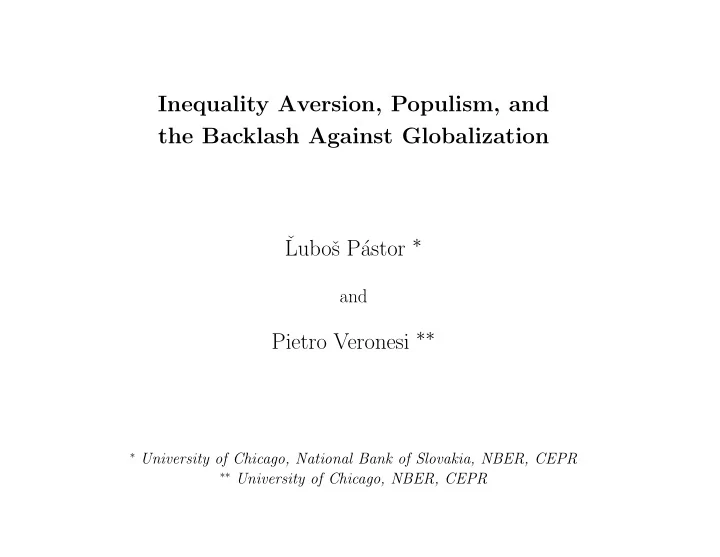
Inequality Aversion, Populism, and the Backlash Against Globalization ˇ Luboˇ s P´ astor ∗

and

Pietro Veronesi ∗∗

∗ University of Chicago, National Bank of Slovakia, NBER, CEPR ∗∗ University of Chicago, NBER, CEPR

Overview

• Model motivated by the backlash against globalization in

rich western democracies (Brexit, Trump, etc.)

Overview

• Model motivated by the backlash against globalization in

rich western democracies (Brexit, Trump, etc.)

• Pushback against globalization emerges endogenously

– Rational voters’ optimal response to rising inequality

Overview

• Model motivated by the backlash against globalization in

rich western democracies (Brexit, Trump, etc.)

• Pushback against globalization emerges endogenously

– Rational voters’ optimal response to rising inequality

Overview

• Model motivated by the backlash against globalization in

rich western democracies (Brexit, Trump, etc.)

• Pushback against globalization emerges endogenously

– Rational voters’ optimal response to rising inequality – Globalization carries the seeds of its own destruction

Economic Mechanism Global growth ⇓ (heterogeneous risk aversion) Inequality ↑

Economic Mechanism Global growth ⇓ (heterogeneous risk aversion) Inequality ↑ ⇓ (inequality aversion) Backlash

Economic Mechanism Global growth ⇓ (heterogeneous risk aversion) Inequality ↑ ⇓ (inequality aversion) Backlash

• Backlash = Elect a populist, Globalization → Autarky

– Risk sharing: Global → Local – Consumption ↓ but equality ↑

Economic Mechanism Global growth ⇓ (heterogeneous risk aversion) Inequality ↑ ⇓ (inequality aversion) Backlash

• Backlash = Elect a populist, Globalization → Autarky

– Risk sharing: Global → Local – Consumption ↓ but equality ↑

• Heterogeneous risk aversion: Within countries =

⇒ Inequality Across countries = ⇒ Imbalances

Empirical Evidence

• Types of evidence

– Across countries: Vote shares of populist parties + Surveys – Across individuals: Brexit + Trump voters

Empirical Evidence

• Types of evidence

– Across countries: Vote shares of populist parties + Surveys – Across individuals: Brexit + Trump voters

• Evidence largely supports the model

– Countries: More populist if they have ∗ Higher inequality ∗ Higher financial development ∗ Lower current account balance – Individuals: More populist if they are ∗ More risk-averse ∗ More inequality-averse

Model

• Continuum of agents i ∈ [0, 1] in countries k ∈ {US, RoW}

Model

• Continuum of agents i ∈ [0, 1] in countries k ∈ {US, RoW}
• Preferences of agent i ∈ Ik at time t ∈ [0, T]:

Ui

• Cit, V k

t , t

• = e−φt
• C1−γi

it

1 − γi where γi = Risk aversion

Model

• Continuum of agents i ∈ [0, 1] in countries k ∈ {US, RoW}
• Preferences of agent i ∈ Ik at time t ∈ [0, T]:

Ui

• Cit, V k

t , t

• = e−φt
• C1−γi

it

1 − γi − ηiV k

t

• where

V k

t = Var

• Cit

Ck

t

| i ∈ Ik

• = Inequality in country k

γi = Risk aversion ηi = Inequality aversion (≈ anti-elitism, “envy of the rich”)

Inequality Aversion

• Evidence

– Experiments – Surveys

Source: Harvard Business Review

Model

• Continuum of agents i ∈ [0, 1] in countries k ∈ {US, RoW}
• Preferences of agent i ∈ Ik at time t ∈ [0, T]:

Ui

• Cit, V k

t , t

• = e−φt
• C1−γi

it

1 − γi − ηiV k

t

• where

V k

t = Var

• Cit

Ck

t

| i ∈ Ik

• = Inequality in country k

γi = Risk aversion ηi = Inequality aversion (≈ anti-elitism, “envy of the rich”)

Model

• U.S. agents are less risk-averse than RoW agents

– Interpretation: U.S. more financially developed than RoW

Model

• U.S. agents are less risk-averse than RoW agents

– Interpretation: U.S. more financially developed than RoW

• Technical assumption:

limx→∞ EI[ex/γj | j ∈ IRoW] EI[ex/γi | i ∈ IUS] = 0 Examples:

• 1. γi < γj for all i ∈ IUS, j ∈ IRoW
• 2. U.S. risk tolerance 1

γi ∼ U[a, b], RoW’s 1 γj ∼ U[a, c], with b > c

• 3. Truncated normals for 1

γi in both countries, same truncation

points, same dispersion, higher mean in the U.S.

Model

• Global output: Dt = DUS

t

+DRoW

t

. Its log, δt ≡ log(Dt), follows dδt = µδ dt + σδ dZt where µδ > 0 ⇒ output trends upward

Model

• Global output: Dt = DUS

t

+DRoW

t

. Its log, δt ≡ log(Dt), follows dδt = µδ dt + σδ dZt where µδ > 0 ⇒ output trends upward

• For simplicity, also assume (relaxed later):

DUS

t

Dt = U.S. population share

• Agents share risk in complete markets

– Interpretation 1: Financial contracts (stocks, bonds) – Interpretation 2: Labor contracts (risky, safe jobs)

Model

• Two possible regimes:
• 1. Globalization: Cross-border trade allowed

Global risk sharing

• 2. Autarky: Cross-border trade not allowed

Local risk sharing

Model

• Two possible regimes:
• 1. Globalization: Cross-border trade allowed

Global risk sharing

• 2. Autarky: Cross-border trade not allowed

Local risk sharing

• Both countries hold elections at known time τ ∈ [0, T]
• 1. Mainstream candidate: Keep globalization
• 2. Populist candidate: Move to autarky

– Elections decided by the median voter

Model

• Two possible regimes:
• 1. Globalization: Cross-border trade allowed

Global risk sharing

• 2. Autarky: Cross-border trade not allowed

Local risk sharing

• Both countries hold elections at known time τ ∈ [0, T]
• 1. Mainstream candidate: Keep globalization
• 2. Populist candidate: Move to autarky

– Elections decided by the median voter

• Expropriation not allowed

– Can’t move to autarky if other country suffers consumption loss

Optimal Consumption

• Complete markets =

⇒ Agent i in country k solves max

{Cit} E0

T Ui

• Cit, V k

t , t

• dt
• s.t. E0

T πk

t Cit dt

• = wi

where πk

t = state price density, wi = initial endowment

Optimal Consumption

• Complete markets =

⇒ Agent i in country k solves max

{Cit} E0

T Ui

• Cit, V k

t , t

• dt
• s.t. E0

T πk

t Cit dt

• = wi

where πk

t = state price density, wi = initial endowment

• Result: C∗

it = f(γi, πk t )

– High-γi agents choose consumption less sensitive to shocks

Equilibrium under Globalization

• Market clearing: Dt =
• i∈I Cit di. Solve for πt = πUS

t

= πRoW

t

.

Equilibrium under Globalization

• Market clearing: Dt =
• i∈I Cit di. Solve for πt = πUS

t

= πRoW

t

.

• Result: Low-γi agents grow disproportionately rich

– Their consumption shares grow with output

Cit Ck

t

↑ in δt iff γi < γk(δt) – Benefits of growth accrue increasingly to “elites”

Equilibrium under Globalization

• Market clearing: Dt =
• i∈I Cit di. Solve for πt = πUS

t

= πRoW

t

.

• Result: Low-γi agents grow disproportionately rich

– Their consumption shares grow with output

Cit Ck

t

↑ in δt iff γi < γk(δt) – Benefits of growth accrue increasingly to “elites”

• Result: Fraction of agents who grow richer declines with output

δt ↑ = ⇒ γk(δt) ↓ – The ranks of elites are shrinking

5 10 15 20 25 30 35 40 0.2 0.4 0.6

• A. US Consumption Distribution

Global log GDP = 1 Global log GDP = 1.5 Global log GDP = 2 Global log GDP = 3

1 2 3 4 5 0.5 1 1.5

• B. US Consumption Share Distribution

Global log GDP = 1 Global log GDP = 1.5 Global log GDP = 2 Global log GDP = 3

Equilibrium under Globalization

• Result: Inequality V k increases, without bounds, as output grows.

So does the skewness of consumption shares. = ⇒ Inequality grows with output, driven by elites’ consumption

1 2 3

Global log output t

0.2 0.4 0.6

Variance Panel A. Inequality in US

1 2 3

Global log output t

0.2 0.4 0.6

Variance Panel B. Inequality in RoW

1 2 3

Global log output t

1 2 3

Skewness Panel C. Skewness in US

1 2 3

Global log output t

1 2 3

Skewness Panel D. Skewness in RoW

Equilibrium under Globalization

• Result: U.S. runs a current account deficit, RoW runs a surplus.
• i∈IUS Cit di > DUS

t

,

• i∈IRoW Cit di < DRoW

t

0.5 1 1.5 2 2.5 3

Global log output

• 20
• 10

10 20 30 40 50 60

Percent of local GDP

US RoW

Equilibrium under Autarky

• Market clearing: Dk

t =

• i∈Ik Cit di , for k ∈ {US, RoW}

= ⇒ Solve for πUS

t

= πRoW

t

Equilibrium under Autarky

• Market clearing: Dk

t =

• i∈Ik Cit di , for k ∈ {US, RoW}

= ⇒ Solve for πUS

t

= πRoW

t

• Result: U.S. inequality is lower under autarky than under
• globalization. The opposite is true for RoW.

1 2 3

Global log output t

0.2 0.4 0.6

Variance Panel A. Inequality in US

Globalization Autarky

1 2 3

Global log output t

0.2 0.4 0.6

Variance Panel B. Inequality in RoW

Globalization Autarky

Elections

• Result: There exists output level δ such that for any δτ > δ,

the populist wins the U.S. election. The Populist Vote Share

0.5 1 1.5 2 2.5 3

Global log output t

10 20 30 40 50 60 70 80 90 100

Percent

Elections

• At time τ, agents in country k vote, comparing expected utilities

Eτ T

τ

e−φ(s−τ)

• C1−γi

is

1 − γi − ηiV k

s

• ds
• under the two candidates (mainstream, populist)

Elections

• At time τ, agents in country k vote, comparing expected utilities

Eτ T

τ

e−φ(s−τ)

• C1−γi

is

1 − γi − ηiV k

s

• ds
• under the two candidates (mainstream, populist)
• Result:

For any U.S. agent i with ηi > 0, there exists δi such that for any δτ > δi, the agent votes populist.

Elections

• At time τ, agents in country k vote, comparing expected utilities

Eτ T

τ

e−φ(s−τ)

• C1−γi

is

1 − γi − ηiV k

s

• ds
• under the two candidates (mainstream, populist)
• Result:

For any U.S. agent i with ηi > 0, there exists δi such that for any δτ > δi, the agent votes populist.

• Intuition: Consumption-equality tradeoff

– Move to autarky = ⇒ Cit ↓ but V US

t

↓

Elections

• At time τ, agents in country k vote, comparing expected utilities

Eτ T

τ

e−φ(s−τ)

• C1−γi

is

1 − γi − ηiV k

s

• ds
• under the two candidates (mainstream, populist)
• Result:

For any U.S. agent i with ηi > 0, there exists δi such that for any δτ > δi, the agent votes populist.

• Intuition: Consumption-equality tradeoff

– Move to autarky = ⇒ Cit ↓ but V US

t

↓ – δt ↑ = ⇒ Marginal utility of Cit ↓ = ⇒ Equality dominates ∗ Equality is a luxury good

Can Redistribution Save Globalization?

• Social planner would preserve globalization

– But market equilibrium = social planner solution (externality)

Can Redistribution Save Globalization?

• Social planner would preserve globalization

– But market equilibrium = social planner solution (externality)

• Result:

Any redistributive policy {Ti,t(δt)} s.t.

• Tidi = 0 is

equivalent to a redistribution of initial endowments wi – With complete markets, redistributive policies are “traded away”

• Agent i’s budget constraint under redistribution:

E0 T πk

t Cit dt

• = wi + E0

T πk

t Tit dt

• To implement redistributive policy {Ti,t(δt)}, augment agent i’s

initial endowment by ˜ wi = E0 T

0 πk t Tit dt

• . Note:
• ˜

widi = 0.

Can Redistribution Save Globalization?

• For tractability, we consider initial endowments of the form

wi = eψi E0 T e−φt+

• gk

t −y

• /γi−gk

t dt

• Increase y =

⇒ Redistribute wi from low-γi to high-γi agents – From those who benefit from globalization to those who lose

2 4 6 8 10

Redistribution Coefficient y

• 0.5

0.5 1

Corr(wi, i)

Can Redistribution Save Globalization?

• Result: For any redistributive policy y there exists δ such that

for any δτ > δ, the populist wins the U.S. election. = ⇒ For any given y, when τ is large enough, the populist wins

Can Redistribution Save Globalization?

• Result: For any redistributive policy y there exists δ such that

for any δτ > δ, the populist wins the U.S. election. = ⇒ For any given y, when τ is large enough, the populist wins

Redistribution Coefficient y

2 4 6 8 10

Redistribution Coefficient y

2.1 2.2 2.3 2.4

• Result: Redistribution can delay the populist win but not forever

Evidence: Which Countries Are Populist?

• Predictions: Populism is stronger in countries with

– Higher inequality – Lower current account balance – Higher financial development

Evidence: Which Countries Are Populist?

• Predictions: Populism is stronger in countries with

– Higher inequality – Lower current account balance – Higher financial development

• Examine a recent cross-section of rich countries
• Measure populism in four ways

– Vote share of populist parties in recent elections ∗ Populist = 1. Nationalist, 2. Anti-immigrant, 3. Anti-elite ∗ Data from ParlGov and 2014 Chapel Hill Survey of Experts – Survey-based support for protectionism; 2013 ISSP data

Vote Share of Nationalist Parties

Panel A. Inequality: Gini Coefficient Panel B. Inequality: Top 10% Share Panel C. Current Account Balance Panel D. Financial Development

Vote Share of Anti-Immigrant Parties

Panel A. Inequality: Gini Coefficient Panel B. Inequality: Top 10% Share Panel C. Current Account Balance Panel D. Financial Development

Vote Share of Anti-Elite Parties

Panel A. Inequality: Gini Coefficient Panel B. Inequality: Top 10% Share Panel C. Current Account Balance Panel D. Financial Development

Support for Protectionism

Panel A. Inequality: Gini Coefficient Panel B. Inequality: Top 10% Share Panel C. Current Account Balance Panel D. Financial Development

Who Are the Populist Voters?

• Result: Agents with higher γi and ηi tend to vote populist

2 3 4 5 6 7

Risk aversion i

0.5 1

Panel A. Risk Aversion

Populist Voters Mainstream Voters

0.5 1 1.5 2

Inequality aversion i

10-3 1000 2000

Panel B. Inequality Aversion

Populist Voters Mainstream Voters

100 200 300 400 500 600

Wealth at

0.005 0.01

Panel C. Wealth at

Populist Voters Mainstream Voters

Evidence: Who Are the Populist Voters?

• Use survey data on Brexit and Trump voters

– Brexit: 2014-2018 British Election Study, panel data – Trump: 2016 Cooperative Congressional Election Survey

• Empirical proxies:

– Risk aversion ∗ Brexit: Income, Education, WillingToTakeRisk, Religious ∗ Trump: Income, Education – Inequality aversion ∗ Brexit: Income, Religious, LeftRight, InequalityBad, Politi- ciansFavorTheRich, LawFavorsTheRich, DoNotTrustExperts ∗ Trump: Income, Religious, Republican

Determinants of the Support for Brexit

(1) (2) (3) (4) (5) (6) (7) (8) Income

• 0.09
• 0.06
• 0.06
• 0.06

(-27.04) (-15.04) (-7.86) (-7.28) Education

• 1.27
• 1.22
• 0.65
• 0.55

(-60.29) (-44.27) (-12.57) (-9.83) WillingnessToTakeRisk 0.11 0.21 0.17 0.20 (7.86) (10.97) (4.98) (5.54) LeftRight 0.44 0.47 0.45 0.42 (47.88) (41.71) (35.20) (31.07) Religious 0.31 0.15 0.16 0.11 (8.52) (3.43) (3.16) (2.07) InequalityBad 0.12

• 0.04
• 0.03
• 0.02

(3.40) (-0.89) (-0.62) (-0.37) PoliticiansFavorTheRich 0.29 0.27 0.30 (10.82) (8.73) (9.34) LawFavorsTheRich 0.11 0.07 0.08 (3.71) (1.92) (2.17) DoNotTrustExperts 0.78 0.68 0.66 (36.94) (27.76) (25.90) Minority

• 0.54

(-5.53) Age 0.01 (4.23) Gender (Male)

• 0.14

(-2.55) Feminist

• 0.36

(-11.47) Observations 31095 40783 40890 25328 15631 13953 10838 10370 R2 0.02 0.09 0.002 0.11 0.21 0.35 0.36 0.38

Determinants of the Support for Trump

(1) (2) (3) (4) (5) (6) (7) Panel A. Controlling for Republican Dummy Republican 3.06 3.06 3.06 3.05 2.92 2.92 2.86 (95.92) (95.93) (95.83) (94.51) (94.66) (89.32) (84.45) Income

• 0.02

0.06 0.10 0.11 0.08 (-4.64) (3.86) (6.41) (6.70) (4.82) Income2

• 0.002
• 0.01
• 0.01
• 0.005
• 0.004

(-5.72) (-5.11) (-4.85) (-4.43) (-3.80) Education

• 0.27
• 0.26
• 0.24

(-28.72) (-27.31) (-23.82) Religious 0.40 0.37 0.46 (37.84) (32.59) (37.82) Minority

• 1.28

(-34.04) Age 0.01 (14.76) Gender (Male) 0.57 (21.14) Observations 40445 40445 40445 40445 45209 40426 40426 R2 0.32 0.32 0.32 0.33 0.34 0.35 0.40

Determinants of the Support for Trump

(1) (2) (3) (4) (5) (6) (7) Panel B. No Control for Republican Dummy Income

• 0.001

0.10 0.14 0.15 0.12 (-0.27) (7.30) (10.42) (10.52) (8.15) Income2

• 0.0004
• 0.01
• 0.01
• 0.01
• 0.01

(-2.10) (-7.58) (-7.22) (-6.36) (-5.43) Education

• 0.28
• 0.27
• 0.25

(-35.71) (-33.09) (-28.58) Religious 0.53 0.51 0.61 (58.25) (52.02) (57.66) Minority

• 1.59

(-47.71) Age 0.01 (14.54) Gender (Male) 0.47 (20.32) Observations 40456 40456 40456 40456 45222 40437 40437 R2 0.00 0.0001 0.001 0.03 0.08 0.10 0.19

Asset Prices

• Result: Global market share of U.S. stocks increases before

the populist victory.

• Result: U.S. bond yields fall before the populist victory.

0.5 1 1.5 2 2.5 3

Global log output t

50 100

Percent Panel B. Global Market Share of US Stocks

0.5 1 1.5 2 2.5 3

Global log output t

• 10

10 20

Percent Panel C. Bond Yields

US RoW

Global Share of U.S. Stock Market

Extensions = ⇒ Same Conclusions

• Time-varying U.S. output share Ft

– Populist elected if δτ > δ(Fτ), where δ′(Fτ) > 0 – U.S. output share ↓ = ⇒ Populism ↑

• Time-varying population shares

– Immigration from RoW to U.S. = ⇒ Populism ↑

• Higher costs of autarky

– Lower output growth, µδ – Higher output volatility, σδ

Conclusions

• Backlash against globalization arises endogenously in our model

– Rational voters’ optimal response to rising inequality

• Key modeling ingredients:

– Inequality aversion – Heterogeneous risk aversion (within & across countries) – Risk sharing (global vs. local)

• Evidence across countries and voters largely supports the model

– Countries are more populist if they have more inequality, more financial development, and current account deficits – Voters are more populist if more risk- and inequality-averse