Industrial Automation Automation Industrielle Industrielle - PowerPoint PPT Presentation
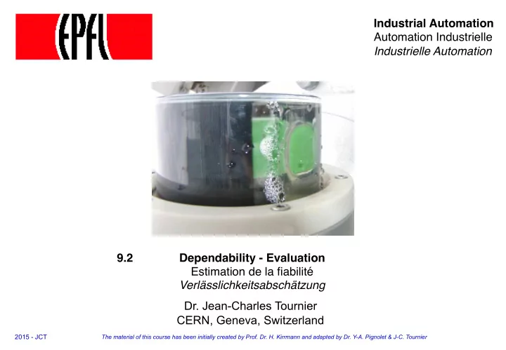
Industrial Automation Automation Industrielle Industrielle Automation 9.2 Dependability - Evaluation Estimation de la fiabilit Verlsslichkeitsabschtzung Dr. Jean-Charles Tournier CERN, Geneva, Switzerland 2015 - JCT The material
Industrial Automation Automation Industrielle Industrielle Automation 9.2 Dependability - Evaluation Estimation de la fiabilité Verlässlichkeitsabschätzung Dr. Jean-Charles Tournier CERN, Geneva, Switzerland 2015 - JCT The material of this course has been initially created by Prof. Dr. H. Kirrmann and adapted by Dr. Y-A. Pignolet & J-C. Tournier
Dependability Evaluation This part of the course applies to any system that may fail. Dependability evaluation ( fiabilité prévisionnelle , Verlässlichkeitsabschätzung ) determines: • the expected reliability, • the requirements on component reliability, • the repair and maintenance intervals and • the amount of necessary redundancy. Dependability analysis is the base on which risks are taken and contracts established Dependability evaluation must be part of the design process, it is quite useless once a system has been put into service. Dependability – Evaluation 9.2 - 2 Industrial Automation
9.2.1 Reliability definitions 9.2.1 Reliability definitions 9.2.2 Reliability of series and parallel systems 9.2.3 Considering repair 9.2.4 Markov models 9.2.5 Availability evaluation 9.2.6 Examples Dependability – Evaluation 9.2 - 3 Industrial Automation
Reliability Reliability = probability that a mission is executed successfully (definition of success? : a question of satisfaction … ) Reliability depends on: • duration ( “ tant va la cruche à l’eau … . ” , " der Krug geht zum Brunnen bis er bricht ) ) • environment: temperature, vibrations, radiations, etc... R(t) 1,0 lim R(t) = 0 t →∞ 25º laboratory 25º 40º vehicle 85º 85º time 1 2 3 4 5 6 Such graphics are obtained by observing a large number of systems, or calculated for a system knowing the expected behaviour of the elements. Dependability – Evaluation 9.2 - 4 Industrial Automation
Reliability and failure rate - Experimental view Experiment: large quantity of light bulbs 100% t remaining good bulbs R(t) time λ aging infancy mature time t + Δ t t Reliability R(t): number of good bulbs remaining at time t divided by initial number of bulbs Failure rate λ (t) : number of bulbs that failed in interval t, t+ Δ t , divided by number of remaining bulbs Dependability – Evaluation 9.2 - 5 Industrial Automation
Bathtube Curve Empirical studies showed that the evolution of the failure rate over time usually follows a “bathtube” curve. Infant Useful life End of life Mortality A typical bathtube curve comprises λ three phases: • Infant mortality • Failure rate is decreasing • Useful life • Failure rate is constant • End of life time • Failure rate is increasing Reminder : a bathtube curve does not depict the failure rate of a single item, but describes the relative failure rate of an entire population of products over time Dependability – Evaluation 9.2 - 6 Industrial Automation
Hardware Failure Hardware failures during a products life can be attributed to the following causes: • Design failures: • This class of failures take place due to inherent design flaws in the system. In a well-designed system this class of failures should make a very small contribution to the total number of failures. • Infant Mortality: • This class of failures cause newly manufactured hardware to fail. This type of failures can be attributed to manufacturing problems like poor soldering, leaking capacitor etc. These failures should not be present in systems leaving the factory as these faults will show up in factory system burn in tests. • Random Failures: • Random failures can occur during the entire life of a hardware module. These failures can lead to system failures. Redundancy is provided to recover from this class of failures. • Wear Out: • Once a hardware module has reached the end of its useful life, degradation of component characteristics will cause hardware modules to fail. This type of faults can be weeded out by preventive maintenance and routing of hardware. Dependability – Evaluation 9.2 - 7 Industrial Automation
Infant Mortality • For critical system, infant mortality is unacceptable • Stress test and burn-in tests should be implemented • Stress tests are used to identify failure root cause (design, process, material) • Burn-in tests are used to identify failure for which root cause can not be found • Both tests are similar, but one is implemented before a massive production (stress test), while the other one is implement on the product leaving the factory (burn-in) • Stress testing • Should be started at the earliest development phases and used to evaluate design weaknesses and uncover specific assembly and materials problems. • The failures should be investigated and design improvements should be made to improve product robustness. Such an approach can help to eliminate design and material defects that would otherwise show up with product failures in the field. • Parameters: temperature, humidity, vibrations, etc. • Burn-in tests • Ensure that a device or system functions properly before it leaves the manufacturing plant • For example, running a new computer for several days before committing it to its real intent • For ships or craft, and in general for complete system, burn-in tests are called shakedown tests Dependability – Evaluation 9.2 - 8 Industrial Automation
Reliability R(t) definition failure good bad Reliability R(t): probability that a system does not enter a terminal state until time t, while it was initially in a good state at time t=0" R(0) = 1; lim R(t) = 0 t →∞ Failure rate λ (t) = probability that a (still good) element fails during the next time unit dt. dR(t) / dt R(t) λ (t) = – definition: R(t) 1 t – λ ( x) dx t 0 R(t) = e 0 MTTF = mean time to fail = surface below R(t) ∞ MTTF = R(t) dt definition: 0 Dependability – Evaluation 9.2 - 9 Industrial Automation
Assumption of constant failure rate λ (t) Reliability = probability of not having failed bathtub aging until time t expressed: childhood by discrete expression (burn-in) mature R (t+ Δ t) = R (t) - R (t) λ (t)* Δ t t by continuous expression simplified R(t) when λ = constant 1 R (t) = e - λ t R(t)= e -0.001 t ( λ = 0.001/h) 0.8 assumption of λ = constant is justified by 0.6 experience, simplifies computations significantly R(t) λ = bathtub 0.4 0.2 MTTF = mean time to fail = surface below R(t) 0 t ∞ 1 MTTF = e - λ t dt = MTTF λ 0 Dependability – Evaluation 9.2 - 10 Industrial Automation
Examples of failure rates To avoid the negative exponentials, λ values are often given in FIT (Failures in Time), 1 1 fit = 10 -9 /h = Element Rating failure rate 114'000 years resistor 0.25 W 0.1 fit capacitor (dry) 100 nF 0.5 fit FIT reports the number of capacitor (elect.) 100 µ F 10 fit expected failures per one billion processor 486 500 fit hours of operation for a device. RAM 4MB 1 fit Flash 4MB 12 fit FPGA 5000 gates 80 fit This term is used particularly by the PLC compact 6500 fit semiconductor industry. digital I/O 32 points 2000 fit analog I/O 8 points 1000 fit battery per element 400 fit VLSI per package 100 fit soldering per point 0.01 fit These figures can be obtained from catalogues such as MIL Standard 217F or from the manufacturer ’ s data sheets. Warning: Design failures outweigh hardware failures for small series Dependability – Evaluation 9.2 - 11 Industrial Automation
MIL HDBK 217 (1) MIL Handbook 217B lists failure rates of common elements. Failure rates depend strongly on the environment: temperature, vibration, humidity, and especially the location: - Ground benign, fixed, mobile - Naval sheltered, unsheltered - Airborne, Inhabited, Uninhabited, cargo, fighter - Airborne, Rotary, Helicopter - Space, Flight Usually the application of MIL HDBK 217 results in pessimistic results in terms of the overall system reliability (computed reliability is lower than actual reliability). To obtain more realistic estimations it is necessary to collect failure data based on the actual application instead of using the generic values from MIL HDBK 217. Dependability – Evaluation 9.2 - 12 Industrial Automation
Failure rate catalogue MIL HDBK 217 (2) Stress is expressed by lambda factors Basic models: – discrete components (e.g. resistor, transistor etc.) λ = λ b p E p Q p A – integrated components (ICs, e.g. microprocessors etc.) λ = p Q p L (C 1 p T p V + C 2 p E ) MIL handbook gives curves/rules for different element types to compute factors, – λ b based on ambient temperature Q A and electrical stress S – p E based on environmental conditions – p Q based on production quality and burn-in period – p A based on component characteristics and usage in application – C 1 based on the complexity – C 2 based on the number of pins and the type of packaging – p T based on chip temperature Q J and technology – p V based on voltage stress Example: λ b usually grows exponentially with temperature Θ A (Arrhenius law) Dependability – Evaluation 9.2 - 13 Industrial Automation
What can go wrong … poor soldering (manufacturing) … broken wire … (vibrations) tin whiskers (lead-free soldering) chip cracking broken isolation (assembly … ) (thermal stress … ) Dependability – Evaluation 9.2 - 14 Industrial Automation
Recommend
More recommend
Explore More Topics
Stay informed with curated content and fresh updates.
