Induction in Isabelle: Lecture 14 1 Notation In lecture 14 we - PDF document
Induction in Isabelle: Lecture 14 1 Notation In lecture 14 we introduced some recursive definitions for lists. Isabelle has most of these already defined in a theory List.thy . This can be found locally at /usr/share/Isabelle/src/HOL There
Induction in Isabelle: Lecture 14 1 Notation In lecture 14 we introduced some recursive definitions for lists. Isabelle has most of these already defined in a theory List.thy . This can be found locally at /usr/share/Isabelle/src/HOL There are some differences in notation and function names: • the empty list is denoted by [ ] • the Cons constructor is denoted by :: • appending two lists is done using the infix operator ”@” • the length of a list is found using the function length The functions butlast , mem and rev have the same names in Isabelle. In lectures we used a rule called replacement . Newer versions of Isabelle have a version of this rule in their theory library, but unfortunately the version on DICE does not. As this rule will be useful in our proofs to come, we prove a generalisation of it below: lemma replacement : [ [ a = b ; c = d ] ] = ⇒ f a c = f b d apply ( erule ssubst )+ apply ( rule refl ) done 2 Recursive Datatypes and Inductive Proofs 2.1 Lists In lecture 14 we proved the associativity of the the append operator by using h :: t -induction on the variable k . In Isabelle, we invoke an inductive proof 1
using a tactic called induct tac . This tactic must be told which variable we are inducting upon, e.g. apply (induct tac k) . Once processed, this command automatically generates two subgoals; our base case and step case to be proved. This can be illustrated by the following proof in Isabelle: lemma assoc-append : k @ ( l @ m ) = ( k @ l ) @ m apply ( induct-tac k ) apply ( subst append-Nil )+ apply ( rule refl ) apply ( subst append-Cons ) apply ( subst append-Cons ) apply ( subst append-Cons ) apply ( rule-tac f = Cons in replacement ) apply ( rule refl ) apply assumption done In proving the associativity of append, we used some of the lemmas from Is- abelle’s library. Remembering the names of all the proved lemmas is difficult and certainly not expected! You should instead be comfortable looking these lemmas up in Isabelle’s theory library (go to /usr/share/Isabelle/src ). It is a useful skill if you ever want to do any serious theorem proving. Luckily, Isabelle adds many of it’s lemmas to the simplifier. So in many proofs you can simply apply simp and Isabelle will automatically prove or simplify the goal. This happens to be the case in our previous inductive proof: lemma assoc-append2 : k @ ( l @ m ) = ( k @ l ) @ m apply ( induct-tac k ) by simp + 3 Reversing a List In the lecture we also looked at a recursive definition to reverse a list. In Isabelle, this could be defined as: consts rev2 :: ′ a list = > ′ a list primrec rev2-Nil : rev2 [] = [] rev2-Cons : rev2 ( x # xs ) = rev2 ( xs ) @ [ x ] We use the keyword primrec to define our function rev2 . This indicates that our function is of the primitive recursive type, as it is guaranteed to terminate due to the fact we always remove a datatype constructor with each call and eventually reach the empty list, which is our unique minimal element. 2
Also notice that we explicitly named the two cases in our definition. This is not essential, but it can be useful. Isabelle does automatically add the definitions as rewrite rules in the simplifier, but for situations when you want to use just those definitions in your proof then you must have given them names. Recall from lecture 14 that we proved a lemma which stated that if we reverse a list twice, we end up with the original list. The proof is shown below along with the extra lemma rev append2 we required: lemma rev-append2 : rev2 ( xs @ ys ) = rev2 ys @ rev2 xs apply ( induct-tac xs ) by simp + lemma rev-rev : rev2 ( rev2 l ) = l apply ( induct-tac l ) apply ( subst rev2-Nil ) apply ( subst rev2-Nil ) apply ( rule refl ) apply ( subst rev2-Cons ) apply ( subst rev-append2 ) apply ( subst rev2-Cons ) apply ( subst rev2-Nil ) apply ( subst append-Nil ) apply ( subst append-Cons ) apply ( subst append-Nil ) apply ( rule-tac f = Cons in replacement ) apply ( rule refl ) apply assumption done If you consult the Isabelle theory List.thy you will notice that a function rev , which reverses lists, already exists. So, we did not need to define rev2 . Using Isabelle’s definition and the the simplifier we could give an alternate proof of the lemma rev rev : lemma rev ( rev l ) = l apply ( induct-tac l ) by simp + 4 Well-founded Recursion in Isabelle Not all recursive functions have a natural primitive recursive definition. When defining this sort of function in Isabelle it is necessary to use the keyword recdef and also explicitly state a suitable measure which will de- crease with every call to the function. This is because Isabelle only accepts total functions . Take, for example, a function which computes the Fibonacci number for a natural number n : 3
consts fib :: nat = > nat recdef fib measure ( λ n . n ) fib 0 = 0 fib ( Suc 0 ) = 1 fib ( Suc ( Suc x )) = fib x + fib ( Suc x ) Notice that we use lambda calculus to map our argument to a measure. For the Fibonacci function fib our measure is that the argument (a natural number) passed to the function decreases with every call. Recursive functions which are not primitive and which take more than one argument, must be defined as curried functions. For example, the function nadd , which adds two natural numbers: consts nadd :: [ nat ∗ nat ] = > nat recdef nadd measure ( λ ( n , m ) . n ) nadd ( 0 , N ) = N nadd (( Suc x ) , N ) = nadd ( x , ( Suc N )) Here we map our argument (a pair of natural numbers) to a measure which states that the first number in the pair must decrease with every call to our recursive function nadd . A property of the fib function is that it is greater than 0 for the successor of every argument we can call it with. This is easily proved in Isabelle using induction: lemma 0 < fib ( Suc n ) apply ( induct-tac n ) by simp + We can prove more complicated lemmas involving Fibonacci numbers. Re- call that the Fibonacci sequence is 0, 1, 1, 2, 3, 5, 8, .... There is a nice fact that the square of a Fibonacci number F n is the product of its immediate neighbours, plus or minus 1 ( ∀ n > 0). For example, 5*5 = 3*8 + 1. How do we prove this? The theory of the naturals doesn’t know about negative numbers, so we write this lemma as: F n * F n +2 ≤ F n +1 * F n +1 + 1 and F n +1 * F n +1 ≤ F n * F n +2 + 1 (Since n is a natural, this statement is for n + 1 > 0, which matches above.) 4
lemma fib-good-neighbours : ( fib n ) ∗ ( fib ( Suc ( Suc n ))) ≤ ( fib ( Suc n )) ∗ ( fib ( Suc n )) + 1 ∧ ( fib ( Suc n )) ∗ ( fib ( Suc n )) ≤ ( fib n ) ∗ ( fib ( Suc ( Suc n ))) + 1 apply ( induct-tac n ) apply simp apply ( simp add : right-distrib left-distrib ) done As mentioned before, it is sometimes difficult to find the rules you need to use in a proof; looking at the source files for the inherited theories can help. The proof of fib good neighbours uses the rewrite rules for distribution of multiplication, which are defined in: /usr/share/Isabelle/src/HOL/Ring and Field.thy As people don’t always want these rules applied, they are not in the default simp set, but they are good to know about when you do need them! This proof also shows that simp can sometimes do such powerful automation that you don’t even have to understand the underlying maths. Can you see why this proof works? Would this proof be clearer if some subgoals were intro- duced? Do you think we can make the formal translation of our lemma more pre- cise? When is F n +1 * F n +1 - F n * F n +2 equal to − 1 and when is it equal to 1? Can we prove this result in Isabelle? The answer is yes, we can prove this in Isabelle. However, so that we can use subtraction, we need to define another Fibonacci function which returns an integer rather than a natural number. We define this new function similar to before, just with different types: consts fibZ :: nat = > int recdef fibZ measure ( λ n . n ) fibZ 0 = 0 fibZ ( Suc 0 ) = 1 fibZ ( Suc ( Suc x )) = fibZ x + fibZ ( Suc x ) Now we can give a more precise formulation of the ”good neighbours” lemma: F n +1 * F n +1 - F n * F n +2 = { +1, if n is even; − 1, if n is odd } To formalize this in Isabelle, we can use the "if .. then" constructor: lemma fibZ-good-neighbours : ( fibZ ( Suc n )) ∗ ( fibZ ( Suc n )) − ( fibZ n ) ∗ ( fibZ ( Suc ( Suc n ))) = ( if (( n mod 2 )= 0 ) then 1 else − 1 ) apply ( induct-tac n ) 5
apply simp apply ( simp add : right-distrib left-distrib ) apply ( case-tac n mod 2 = 0 ) apply simp apply ( simp add : mod-Suc ) apply simp apply ( simp add : mod-Suc ) done Note that the proof uses a new tactic called case tac . This splits the proof into different cases; in this example we have one subgoal with the assump- tion n mod 2 = 0 and another subgoal with the assumption n mod 2 � = 0 . As an exercise for the intrepid (no solution provided, and this will not be examined): restate the previous lemma using ( − 1) n instead of the ”if ... then” construction. The theory Power.thy will be helpful. 6
Recommend
More recommend
Explore More Topics
Stay informed with curated content and fresh updates.
