4 Recurrences As noted in Section 2.3.2, when an algorithm contains - PDF document

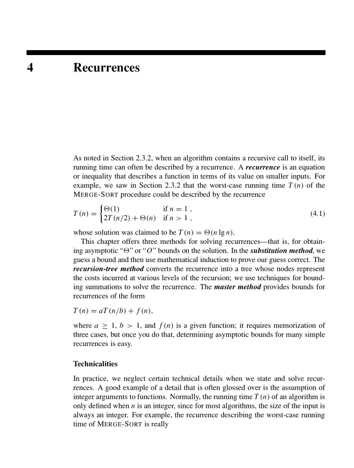
4 Recurrences As noted in Section 2.3.2, when an algorithm contains a recursive call to itself, its running time can often be described by a recurrence. A recurrence is an equation or inequality that describes a function in terms of its value on smaller inputs. For example, we saw in Section 2.3.2 that the worst-case running time T ( n ) of the M ERGE -S ORT procedure could be described by the recurrence � �( 1 ) if n = 1 , T ( n ) = (4.1) 2 T ( n / 2 ) + �( n ) if n > 1 , whose solution was claimed to be T ( n ) = �( n lg n ) . This chapter offers three methods for solving recurrences—that is, for obtain- ing asymptotic “ � ” or “ O ” bounds on the solution. In the substitution method , we guess a bound and then use mathematical induction to prove our guess correct. The recursion-tree method converts the recurrence into a tree whose nodes represent the costs incurred at various levels of the recursion; we use techniques for bound- ing summations to solve the recurrence. The master method provides bounds for recurrences of the form T ( n ) = aT ( n / b ) + f ( n ), where a ≥ 1, b > 1, and f ( n ) is a given function; it requires memorization of three cases, but once you do that, determining asymptotic bounds for many simple recurrences is easy. Technicalities In practice, we neglect certain technical details when we state and solve recur- rences. A good example of a detail that is often glossed over is the assumption of integer arguments to functions. Normally, the running time T ( n ) of an algorithm is only defined when n is an integer, since for most algorithms, the size of the input is always an integer. For example, the recurrence describing the worst-case running time of M ERGE -S ORT is really

4.1 The substitution method 63 � �( 1 ) if n = 1 , T ( n ) = (4.2) T ( ⌈ n / 2 ⌉ ) + T ( ⌊ n / 2 ⌋ ) + �( n ) if n > 1 . Boundary conditions represent another class of details that we typically ignore. Since the running time of an algorithm on a constant-sized input is a constant, the recurrences that arise from the running times of algorithms generally have T ( n ) = �( 1 ) for sufficiently small n . Consequently, for convenience, we shall generally omit statements of the boundary conditions of recurrences and assume that T ( n ) is constant for small n . For example, we normally state recurrence (4.1) as T ( n ) = 2 T ( n / 2 ) + �( n ) , (4.3) without explicitly giving values for small n . The reason is that although changing the value of T ( 1 ) changes the solution to the recurrence, the solution typically doesn’t change by more than a constant factor, so the order of growth is unchanged. When we state and solve recurrences, we often omit floors, ceilings, and bound- ary conditions. We forge ahead without these details and later determine whether or not they matter. They usually don’t, but it is important to know when they do. Experience helps, and so do some theorems stating that these details don’t affect the asymptotic bounds of many recurrences encountered in the analysis of algo- rithms (see Theorem 4.1). In this chapter, however, we shall address some of these details to show the fine points of recurrence solution methods. 4.1 The substitution method The substitution method for solving recurrences entails two steps: 1. Guess the form of the solution. 2. Use mathematical induction to find the constants and show that the solution works. The name comes from the substitution of the guessed answer for the function when the inductive hypothesis is applied to smaller values. This method is powerful, but it obviously can be applied only in cases when it is easy to guess the form of the answer. The substitution method can be used to establish either upper or lower bounds on a recurrence. As an example, let us determine an upper bound on the recurrence T ( n ) = 2 T ( ⌊ n / 2 ⌋ ) + n , (4.4) which is similar to recurrences (4.2) and (4.3). We guess that the solution is T ( n ) = O ( n lg n ) . Our method is to prove that T ( n ) ≤ cn lg n for an appropriate choice of

64 Chapter 4 Recurrences the constant c > 0. We start by assuming that this bound holds for ⌊ n / 2 ⌋ , that is, that T ( ⌊ n / 2 ⌋ ) ≤ c ⌊ n / 2 ⌋ lg ( ⌊ n / 2 ⌋ ) . Substituting into the recurrence yields T ( n ) ≤ 2 ( c ⌊ n / 2 ⌋ lg ( ⌊ n / 2 ⌋ )) + n ≤ cn lg ( n / 2 ) + n = cn lg n − cn lg 2 + n = cn lg n − cn + n ≤ cn lg n , where the last step holds as long as c ≥ 1. Mathematical induction now requires us to show that our solution holds for the boundary conditions. Typically, we do so by showing that the boundary condi- tions are suitable as base cases for the inductive proof. For the recurrence (4.4), we must show that we can choose the constant c large enough so that the bound T ( n ) ≤ cn lg n works for the boundary conditions as well. This requirement can sometimes lead to problems. Let us assume, for the sake of argument, that T ( 1 ) = 1 is the sole boundary condition of the recurrence. Then for n = 1, the bound T ( n ) ≤ cn lg n yields T ( 1 ) ≤ c 1 lg 1 = 0, which is at odds with T ( 1 ) = 1. Consequently, the base case of our inductive proof fails to hold. This difficulty in proving an inductive hypothesis for a specific boundary condi- tion can be easily overcome. For example, in the recurrence (4.4), we take advan- tage of asymptotic notation only requiring us to prove T ( n ) ≤ cn lg n for n ≥ n 0 , where n 0 is a constant of our choosing. The idea is to remove the difficult bound- ary condition T ( 1 ) = 1 from consideration in the inductive proof. Observe that for n > 3, the recurrence does not depend directly on T ( 1 ) . Thus, we can replace T ( 1 ) by T ( 2 ) and T ( 3 ) as the base cases in the inductive proof, letting n 0 = 2. Note that we make a distinction between the base case of the recurrence ( n = 1) and the base cases of the inductive proof ( n = 2 and n = 3). We derive from the recurrence that T ( 2 ) = 4 and T ( 3 ) = 5. The inductive proof that T ( n ) ≤ cn lg n for some constant c ≥ 1 can now be completed by choosing c large enough so that T ( 2 ) ≤ c 2 lg 2 and T ( 3 ) ≤ c 3 lg 3. As it turns out, any choice of c ≥ 2 suffices for the base cases of n = 2 and n = 3 to hold. For most of the recurrences we shall examine, it is straightforward to extend boundary conditions to make the inductive assumption work for small n . Making a good guess Unfortunately, there is no general way to guess the correct solutions to recurrences. Guessing a solution takes experience and, occasionally, creativity. Fortunately, though, there are some heuristics that can help you become a good guesser. You can also use recursion trees, which we shall see in Section 4.2, to generate good guesses.

4.1 The substitution method 65 If a recurrence is similar to one you have seen before, then guessing a similar solution is reasonable. As an example, consider the recurrence T ( n ) = 2 T ( ⌊ n / 2 ⌋ + 17 ) + n , which looks difficult because of the added “17” in the argument to T on the right- hand side. Intuitively, however, this additional term cannot substantially affect the solution to the recurrence. When n is large, the difference between T ( ⌊ n / 2 ⌋ ) and T ( ⌊ n / 2 ⌋+ 17 ) is not that large: both cut n nearly evenly in half. Consequently, we make the guess that T ( n ) = O ( n lg n ) , which you can verify as correct by using the substitution method (see Exercise 4.1-5). Another way to make a good guess is to prove loose upper and lower bounds on the recurrence and then reduce the range of uncertainty. For example, we might start with a lower bound of T ( n ) = �( n ) for the recurrence (4.4), since we have the term n in the recurrence, and we can prove an initial upper bound of T ( n ) = O ( n 2 ) . Then, we can gradually lower the upper bound and raise the lower bound until we converge on the correct, asymptotically tight solution of T ( n ) = �( n lg n ) . Subtleties There are times when you can correctly guess at an asymptotic bound on the so- lution of a recurrence, but somehow the math doesn’t seem to work out in the in- duction. Usually, the problem is that the inductive assumption isn’t strong enough to prove the detailed bound. When you hit such a snag, revising the guess by subtracting a lower-order term often permits the math to go through. Consider the recurrence T ( n ) = T ( ⌊ n / 2 ⌋ ) + T ( ⌈ n / 2 ⌉ ) + 1 . We guess that the solution is O ( n ) , and we try to show that T ( n ) ≤ cn for an appropriate choice of the constant c . Substituting our guess in the recurrence, we obtain T ( n ) c ⌊ n / 2 ⌋ + c ⌈ n / 2 ⌉ + 1 ≤ = cn + 1 , which does not imply T ( n ) ≤ cn for any choice of c . It’s tempting to try a larger guess, say T ( n ) = O ( n 2 ) , which can be made to work, but in fact, our guess that the solution is T ( n ) = O ( n ) is correct. In order to show this, however, we must make a stronger inductive hypothesis. Intuitively, our guess is nearly right: we’re only off by the constant 1, a lower- order term. Nevertheless, mathematical induction doesn’t work unless we prove the exact form of the inductive hypothesis. We overcome our difficulty by subtracting a lower-order term from our previous guess. Our new guess is T ( n ) ≤ cn − b ,