In Situ I/O Processing: A Case for In Situ I/O Processing: A Case - PowerPoint PPT Presentation
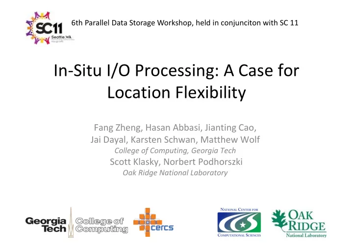
6th Parallel Data Storage Workshop, held in conjunciton with SC 11 In Situ I/O Processing: A Case for In Situ I/O Processing: A Case for Location Flexibility Location Flexibility Fang Zheng, Hasan Abbasi, Jianting Cao, F Zh H Abb i Ji i
6th Parallel Data Storage Workshop, held in conjunciton with SC 11 In ‐ Situ I/O Processing: A Case for In Situ I/O Processing: A Case for Location Flexibility Location Flexibility Fang Zheng, Hasan Abbasi, Jianting Cao, F Zh H Abb i Ji i C Jai Dayal, Karsten Schwan, Matthew Wolf College of Computing, Georgia Tech College of Computing, Georgia Tech Scott Klasky, Norbert Podhorszki Oak Ridge National Laboratory 1
I/O Bottleneck on High End Machines I/O Bottleneck on High ‐ End Machines • Scientific simulation and • I/O subsystem is not catching up Scientific simulation and I/O subsystem is not catching up analysis are data ‐ intensive – capacity mismatching between computation vs. I/O – complicated I/O pattern – shared resource contention Machine Peak Flops Peak I/O Flop/byte bandwidth Jaguar Cray XT5 2.3 Petaflops 120GB/sec 191666 Franklin Cray XT4 352 Teraflops 17GB/sec 20705 Hopper Cray XE6 1.28 Petaflops 35GB/sec 36571 Intrepid BG/P p 557 Teraflops p 78GB/sec 7141 Simulation and analysis spends significant portion of runtime waiting for I/O to finish! portion of runtime waiting for I/O to finish! 2 cite
What is In Situ I/O Processing? What is In ‐ Situ I/O Processing? • Process/analyze simulation output data before data hits disks, during simulation time g Simulation Si l ti A Analysis l i PFS PFS remove the bottleneck! Simulation Analysis 3
Why In Situ I/O Processing? Why In ‐ Situ I/O Processing? • Get around I/O bottleneck by reducing file I/O • Get around I/O bottleneck by reducing file I/O – Reduce data movement along I/O hierarchy – Extract insights from data in a timely manner – Prepapre data better for later analysis p p y – Better end ‐ to ‐ end performance and cost 4
Placement of In Situ Analytics Placement of In ‐ Situ Analytics • • Active R&D efforts Active R&D efforts – Active Storage (recently ANL and PNNL) – Hercules/Quakeshow (CMU&UCDavis&UTAustin&PSC) – ADIOS/DataStager/PreDatA (GT&ORNL) ADIOS/DataStager/PreDatA (GT&ORNL) – DataSpaces (Rutgers&ORNL) – Nessie (Sandia) – GLEAN (ANL) – GLEAN (ANL) – Functional partitioning (ORNL&VT&NCSU) – HDF5/DSM (ETH&CSCS) – ParaView co ‐ processing library (ParaView) ParaView co processing library (ParaView) – VisIt remote visualization (VisIt) – In ‐ situ indexing (LBL), compression (NCSU), etc. • Question: Where should I run In ‐ situ analysis? Question: Where should I run In situ analysis? – Inline with simulation? – Seperate core? – Seprate staging nodes? p g g – I/O servers? – Offline? 5
Placement Matters! Placement Matters! • Placement of In ‐ situ I/O processing have significant impact on performance and cost g p p – How resource is allocated between simulation and analysis analysis – How data is moved between simulation and analysis (interconnect shared memory etc ) analysis (interconnect, shared memory, etc.) – Resource contention effect 6
Flexible Placement is Important Flexible Placement is Important • No one place fits everything – Diverse characteristics of simulaiton and analytics y – Machine parameters – Resource availability Resource availability • Understanding how placement decision affects performance and cost is valuable for end ‐ users 7
Contributions of This Paper Contributions of This Paper • A (Simple) performance model to reason about placement p – Capable of comparing performance and cost of different placements different placements • Application case study ‐‐ Pixie3D I/O Pipeline – Placement makes huge difference in performance and cost – Empirically validate the model 8
Performance and Cost Metrics Performance and Cost Metrics • Performance Metric – Total Execution Time of both simulation and analysis • Cost Metric • Cost Metric – CPU hours charged for simulation and analysis 9
Performance Modeling Performance Modeling • Scenario: – Simulation periodically generate output data and p y g p pass to analyis component – Analysis process the simulation output data on a Analysis process the simulation output data on a per ‐ timestep basis Simulation Simulation Analysis Analysis 10
Performance Modeling Performance Modeling • Place analysis in a staging area vs. inline with simulation? In Staging Area: Inline with simulation: - Simulation runs on Psim nodes Simulation runs on Psim nodes - Both simulation and analysis run on Both simulation and analysis run on - Analysis runs on another Pa nodes the same Psim nodes - Space partition ( Psim + Pa ) nodes - Simulation nodes perform analysis between simulation and analysis between simulation and analysis inline synchronously on Psim nodes inline synchronously on Psim nodes - Pass data through interconnect - Simulation and analysis share Psim nodes in time Simulation Simulation Analysis A Analysis l i Psim nodes Pa nodes Psim nodes
Performance Modeling Performance Modeling • Key parameters Psim Total number of nodes on which simulation is run Pa Total number of nodes in staging area (if present) Simulation’s wall-clock time between two Tsim ( P ) consecutive I/O actions when running on P nodes Analysis’ wall-clock time for processing one Ta ( P ) simulation output step when running on P nodes K Total number of I/O dumps p Tsend Simulation-side visible data movement time Trecv Trecv Staging node-side visible data movement time Staging node side visible data movement time s Slowdown factor of simulation 12
Performance Modeling Performance Modeling • Total execution time Simulation Tinit Tsim Ta Tsim Ta Tsim Ta … Time = × + Tinline K [ Tsim ( Psim ) Ta ( Psim )] Simulation Tinit Tsim x s Ts Tsim x s Ts Tsim x s Ts … Staging Area Tinit wait Tr Ta wait Tr Ta wait Tr Ta Time = × × + + Tstaging K max{ Tsim ( Psim ) s Tsend , Trecv Ta ( Pa )} Pipeline effect of simulation and analysis Slowdown factor of simulation (s>=1) 13
Performance Modeling Performance Modeling • Performance comparison of inline vs. staging Let α =Pa/Psim (size of staging area as percentage of total simulation nodes) (size of staging area as percentage of total simulation nodes) β =Ta(Psim)/ Tsim(Psim) (analysis time as percentage of simulation time on Psim nodes) ( y p g ) since × + + × α > × max{ Tsim ( Psim ) s Tsend , Trecv Ta ( Psim )} Tsim ( Psim ) s There is a upper bound: 14
Performance Modeling Performance Modeling • What does the model say? – Total execution time is (1+ β ) if running analysis ( ) g y inlne with simulation on Psim nodes – If we can use α % additional nodes as staging area to If we can use α % additional nodes as staging area to offload the analysis to staging area – If co ‐ running staging area slows down simulation by If co running staging area slows down simulation by a factor of s – Then the speedup of such offloading is bounded by Th h d f h ffl di i b d d b 15
Performance Modeling Performance Modeling • Comparing Cost of Staging vs. Inline • Cost (inline)=Tinline x Psim ( ) • Cost (staging) = Tstaging x (Psim+Pa) • We want to know the cost efficiency of using W t t k th t ffi i f i additional staging area to offload analysis • Does α % of additional nodes leads to α % improvement in Speedup? 16
Performance Model Performance Model • Key to achieve good speedup and efficiency – No slowdown: s =1 – Tsend =0 – Tsim ( Psim )> Trecv + Ta ( Pa ) – Ta ( P ) scales sub ‐ linearly with P ( Ta ( P )x P decrease with P ) speedup (1 β )/ (1+ β )/s α 1 17 0 α 0 β 0 (1+ β )/s-1 1
Performance Model Performance Model • Not cost ‐ efficient to offload linear ‐ scalable Not cost efficient to offload linear scalable analysis: – Ta ( P ) x P doesn’t change Ta ( P ) x P doesn’t change – Offloading only increase data movement cost speedup d (1+ β )/s α α 1 1 α 0 (1+ β )/s-1 1 18
Performance Model Performance Model • When the minimum size of the staging area When the minimum size of the staging area ( α 0 ), is larger than (1+ β )/ s ‐ 1, then offloading is always in efficient always in ‐ efficient speedup (1+ β )/s α 1 1 19 0 (1+ β )/s-1 α 0 1
Application Case Study Application Case Study • Pixie3D In ‐ Situ I/O Pipeline – Pixie3D MHD simulation – Pixplot: diagnostic analysis – Paraview server: contour plotting Paraview server: contour plotting – Implement with ADIOS/PreDatA middleware 20
Pixie3D Performance Pixie3D Performance • Scalability 100 onds) 10 Time (Seco 1 Pixie3D Simulation Pixplot Analysis File Write 0.1 512 512 1024 1024 2048 2048 4096 4096 8192 8192 Number of cores - Pixplot analysis and I/.O scales worse than Pixie3D simulation, so placing inline Would hurt scalability. - Offloading to a staging area may get good speedup and efficiency 21
Pixie3D Performance Pixie3D Performance • Time Breakdown • Run Pixie3D on 8192 cores, Pixplot on 64 cores , p - Using 0 78% additional nodes as staging area offloading Pixplot and I/O - Using 0.78% additional nodes as staging area, offloading Pixplot and I/O to staging area increases performance by 33% - The speedup is within 96% of upper bound 22
Recommend
More recommend
Explore More Topics
Stay informed with curated content and fresh updates.
