In-operation subspace-based covariance-driven structural - PowerPoint PPT Presentation

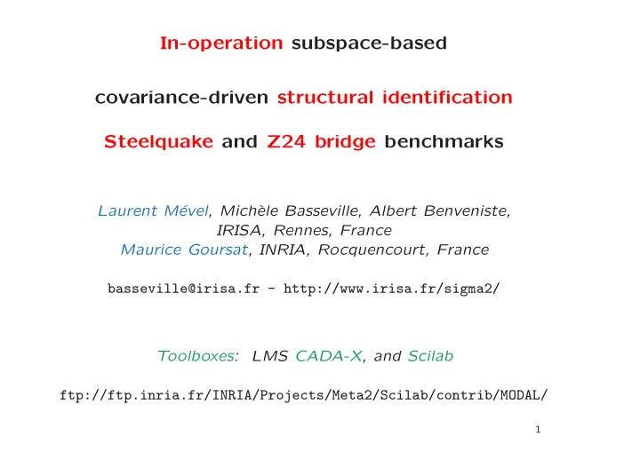
In-operation subspace-based covariance-driven structural identification Steelquake and Z24 bridge benchmarks Laurent M´ evel, Mich` ele Basseville, Albert Benveniste, IRISA, Rennes, France Maurice Goursat, INRIA, Rocquencourt, France basseville@irisa.fr - http://www.irisa.fr/sigma2/ Toolboxes: LMS CADA-X, and Scilab ftp://ftp.inria.fr/INRIA/Projects/Meta2/Scilab/contrib/MODAL/ 1

Problem : In-operation modal identification of structures • The excitation is typically: – natural, not controlled. – not measured: ∗ buildings, bridges, offshore structures, ∗ rotating machinery, ∗ cars, trains, aircrafts. – nonstationary (e.g., turbulent). • How to merge multiple measurements setups e.g. in case of moving sensors? 2

Identification and merging • Output-only eigenstructure identification, • In the presence of nonstationary excitation, • Handling moving sensor pools, with some reference sensors. Wanted: • Avoid merging identification results from the different pools, • Merge the data instead, and process them globally, • Use a standard subspace algorithm. 3

Contents – Modelling – Output-only covariance-based subspace identification – Merging multiple measurements setups – Robustness to nonstationary excitation – Numerical results - Steelquake – Numerical results - Z24 bridge 4

Modelling M ¨ Z ( s ) + C ˙  Z ( s ) + K Z ( s ) = ν ( s )          FE model:      Y ( s ) = L Z ( s )     ( Mµ 2 + Cµ + K )Ψ µ = 0 , ψ µ = L Ψ µ  X k +1 = F X k + V k         State space:      Y k = HX k      ∆ F Φ λ = λ Φ λ , ϕ λ = H Φ λ e δµ = λ , ψ µ = ϕ λ � �� � � �� � modes mode shapes 5

Output-only covariance-based subspace identification   R 0 R 1 R 2 . . .       R 1 R 2 R 3 . . .   ∆    Y k Y T   R i = E , H =      k − i   R 2 R 3 R 4 . . .       � �� � . . ... .   ok if stationary ! . . .  . . .    R i = H F i G , G ∆    X k Y T = E  k   H   O ∆ , C ∆ HF � � G F G F 2 G . . .   = =     HF 2       . .   . H = O C , H − → ( H, F ) − → ( λ, ϕ λ ) → O − 6

Implementation   ˆ ˆ ˆ R 0 R 1 R 2 . . .     ˆ ˆ ˆ = 1   N R 1 R 2 R 3 . . .   ∆ k =1 Y k Y T ˆ ˆ   R i � , H =   k − i   ˆ ˆ ˆ R 2 R 3 R 4 . . . N       . . . ... � �� �   . . .  . . .  ok when nonstationary ! SVD ( ˆ → ˆ → ( ˆ H, ˆ → (ˆ H ) + truncation − F ) − λ, ˆ ϕ λ ) O −    ∆ 1 0 O = U ∆ 1 / 2 H = U ∆ W T = U  W T ; ˆ ˆ     1   0 ∆ 0 O ↑ p ( H, F ) = O p ( H, F ) F det( F − λ I ) = 0 , F Φ λ = λ Φ λ , ϕ λ = H Φ λ 7

Merging multiple measurements setups       Y (0 , 1) Y (0 , 2) Y (0 ,J )       k k k       . . .             Y (1) Y (2) Y ( J )                   k k k � �� � � �� � � �� � Record 1 Record 2 Record J  X ( j ) F X ( j ) + V ( j )    =    k +1 k k                Y (0 ,j ) = H 0 X ( j )    ( the reference ) k k                Y ( j ) = H j X ( j )  ( sensor pool n o j )       k k   T T = E Y (0 ,j ) Y (0 ,j ) = E Y ( j ) Y (0 ,j ) R 0 ,j R j ∆ ∆ , i k k − i i k k − i T T E Y ( j ′ ) E Y ( j ) Y ( j ) Y ( j ) ( j � = j ′ ) not available not used , k k − i k k − i 8

Stationary excitation T cov V ( j ) = E X ( j ) Y (0 ,j ) G ∆ = Q , k k k = H 0 F i G i = H j F i G R 0 ,j R j ∆ = R 0 i , i   R 0   H 0 i         R 1   H 1     = H F i G , ∆ H ∆ R π    i  = =     . .   i . .   .  .               R J  H J     i Nonstationary excitation T cov V ( j ) = E X ( j ) Y (0 ,j ) ∆ = Q j , G j k k k = H 0 F i G j , i = H j F i G j R 0 ,j R j i Hint: right renormalization of the covariances . 9

Robustness to nonstationary excitation Time-varying excitation within each record cov V ( j ) = Q k k Approximate factorization of covariances R i ≈ H F i ˆ ˆ G T − 1 ˆ ˆ Consistency : F T → F, H → H Combination of: • the key factorization property of the covariances, • the averaging operation underlying covariance computation, allows to cancel out nonstationarities in the excitation. 10

Numerical results - Steelquake Estimated modes - Classical subspace identification Mode 1 2 3 4 5 6 7 8 Freq.(Hz) 3.1 3.92 6.1 9.68 10.8 12.27 13.0 17.7 Dir. X Y Y Y X Z Z Z 11

12 Frequency ♦ × ∆ ♦ ♦ ∆ ∆ × ♦ ⊕ × × 25 25 25 25 25 25 × ◊ × ♦ × ◊ ◊ ∆ × × ♦ ♦ ◊ × ∆ × ⊕ ♦ ♦ ♦ ♦ ♦ ♦ × ♦ ♦ ♦ ∆ ∆ ∆ × Twelve sensors (all except sensors 3, 7, 10) ( Q 09 − 1 ). ◊ × × ◊ ∆ × ⊕ ◊ ♦ ⊕ ♦ ⊕ ♦ ♦ ⊕ × ◊ ∆ × ♦ ◊ ∆ ⊕ ◊ ♦ ◊ × ◊ × ♦ × × × ◊ ♦ × ◊ ♦ ∆ ∆ ∆ ♦ ♦ × × ⊕ ⊕ ⊕ ∆ ◊ ♦ ⊕ ◊ ♦ ◊ × + ◊ × ⊕ ⊕ × ⊕ ♦ ⊕ ⊕ ♦ × ⊕ ♦ ♦ ♦ ⊕ ∆ ♦ ♦ × × ⊕ ⊕ ♦ ♦ ♦ ◊ ∆ ◊ ⊕ ♦ × ◊ ♦ ♦ ♦ ◊ ◊ ♦ ◊ ♦ ⊕ 20 20 20 20 20 20 ◊ ◊ ⊕ × × ⊕ × ⊕ ⊕ × ⊕ ⊕ × ⊕ ⊕ ⊕ × ♦ × ⊕ ♦ + + + + + + + + + + + + + + + + + + + + + + + + + + ∆ + + × + + × ⊕ × × × × × × × × ♦ ♦ × × × × × × × × × × × + × × × × × × × + ♦ 19.09 ⊕ ⊕ ♦ × ∆ ◊ ⊕ ⊕ ∆ ∆ ◊ ♦ ⊕ ♦ ◊ ⊕ ⊕ + + + + + + + + + + + + + + + + + + + + + ⊕ × × × + ∆ × × × × × × × × × × × × ♦ × × × × × ⊕ × × × × × × ◊ ∆ ∆ 17.74 × ◊ ⊕ ◊ ∆ ◊ ◊ ∆ ∆ ♦ ♦ ∆ × × ⊕ ♦ ◊ ⊕ ∆ ∆ ∆ × × × ♦ × × × × × × × 15 15 15 15 15 15 ♦ ⊕ × + ⊕ × ∆ ∆ × ∆ ∆ ⊕ ◊ ◊ × ♦ ∆ ∆ × ⊕ ∆ ◊ + + + + + 13.1 + + + + + + + + + + + ◊ + + + + + + + + + + + + + + + + ♦ + + ⊕ × + + + + ⊕ × + + + + + + + + + + ⊕ ⊕ × + + × × × × × + + × × × × × × × ⊕ × × + × × × × × × × + + + + × ⊕ × + + + + + + + + + + ⊕ ⊕ ◊ ♦ 12.98 × + + ⊕ + + + + + + + + + + + + + + + + ∆ × + + + + ⊕ + + + + × × ∆ × × × × × × × × × × × × + × × × + × × × × ◊ + ∆ ♦ ⊕ 12.3 ◊ + + + + + + + + + + + + + + + + + + + ⊕ × ∆ × × × × + + + × × + + + + × × ♦ × × ◊ ⊕ ⊕ + ◊ 11.8 ◊ ⊕ ♦ ⊕ + + + + + + + + + + + + + + + + + ⊕ × × + + × × × ⊕ × × + × + × × × × × × × ⊕ + + + + + + + + ∆ + + + ⊕ + + + + + + + + + + + + + + + + + + × 11.13 × × + + + + + + + + + + + + + + + + + ◊ + + + + + + + + + + + × × ⊕ ◊ ∆ ♦ 10.81 ∆ ⊕ ∆ ♦ × ⊕ × ♦ × × × × ⊕ × ⊕ 10 10 10 10 10 10 ∆ + ∆ ♦ ⊕ ◊ × ♦ ♦ ♦ ∆ ♦ ∆ ⊕ ♦ ∆ ∆ ∆ × ♦ ♦ ♦ + + + + + + + + + + + + + + + + + + + + + ⊕ + + × ∆ + × + + + + + + + + + + + + × + + + + + × ♦ ♦ 6.13 ◊ ◊ ⊕ ∆ × ∆ ♦ ♦ ◊ ∆ ∆ ◊ 5 5 5 5 5 5 ♦ ♦ ♦ × ∆ ♦ ∆ ⊕ ∆ × ∆ ♦ + + + + + + + + ◊ + + + ∆ + + ◊ + + + × ◊ ⊕ + × × × × + × × + × × ⊕ ♦ ⊕ ◊ 3.9 × ∆ + × + × ◊ + + + + + + + + + × + + + + + × ⊕ × ∆ ◊ ♦ + + + + + + + + + Order ∆ 0 0 0 0 0 0 2 2 2 2 2 2 7 7 7 7 7 7 12 12 12 12 12 12 17 17 17 17 17 17 22 22 22 22 22 22 27 27 27 27 27 27 32 32 32 32 32 32 37 37 37 37 37 37