Images Debugging Black and white image is a 2D matrix. Add print - PDF document

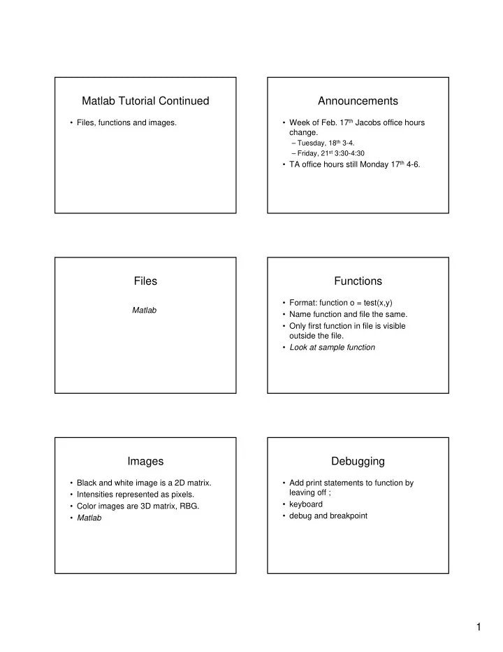
Matlab Tutorial Continued Announcements • Week of Feb. 17 th Jacobs office hours • Files, functions and images. change. – Tuesday, 18 th 3- 4. – Friday, 21 st 3:30 - 4:30 • TA office hours still Monday 17 th 4- 6. Files Functions • Format: function o = test(x,y) Matlab • Name function and file the same. • Only first function in file is visible outside the file. • Look at sample function Images Debugging • Black and white image is a 2D matrix. • Add print statements to function by leaving off ; • Intensities represented as pixels. • keyboard • Color images are 3D matrix, RBG. • debug and breakpoint • Matlab 1

Conclusions Linear Filtering • About modifying pixels based on • Quick tour of matlab , you should teach neighborhood. Local methods simplest. yourself the rest. We’ll give hints in • Linear means linear combination of problem sets. neighbors. Linear methods simplest. • Linear algebra allows geometric • Useful to: manipulation of points. – Integrate information over constant regions. – Scale. • Learn to love SVD. – Detect changes. • Fourier analysis. • Many nice slides taken from Bill Freeman. (Freeman) (Freeman) Convolution • Convolution kernel g, represented as matrix. – it’s associative • Result is: 2

3

4

Filtering to reduce noise Additive noise • Noise is what we’re not interested in. • I = S + N. Noise doesn’t depend on signal. – We’ll discuss simple, low - level noise today: Light fluctuations; Sensor noise; • We’ll consider: = + = I s n with E ( n ) 0 Quantization effects; Finite precision i i i i – Not complex: shadows; extraneous s determinis tic. i objects. ≠ n , n independen t for n n i j i j • A pixel’s neighborhood contains n , n identicall y distribute d information about its intensity. i j • Averaging noise reduces its effect. Does it reduce noise? Average Filter • Intuitively, takes out small variations. • Mask with positive entries, that sum 1. = + σ ˆ F I ( i , j ) I ( i , j ) N ( i , j ) with N(i, j) ~ N(0, ) • Replaces each pixel m / 2 m / 2 1 ∑ ∑ = − − + − − = ˆ with an average of O(i, j) I ( i h , j k ) N ( i h , j k ) 1 1 1 2 m = − = − h m / 2 k m / 2 its neighborhood. 1 1 1 1/9 m / 2 m / 2 m / 2 m / 2 1 ∑ ∑ 1 ∑ ∑ = − − + − − ˆ I ( i h , j k ) N ( i h , j k ) • If all weights are 1 1 1 2 2 m m = − = − = − = − h m / 2 k m / 2 h m / 2 k m / 2 equal, it is called a ˆ N ( i , j ) BOX filter. = ˆ E ( N ( i , j )) 0 σ σ 2 1 ˆ = σ = ⇒ ˆ 2 2 E ( N ( i , j )) m N ( i , j ) ~ N ( 0 , ) (Camps) 2 m m m (Camps) 5

Example: Smoothing by Averaging Matlab Demo of Averaging Smoothing as Inference About Gaussian Averaging the Signal • Rotationally Neighborhood for symmetric. averaging. • Weights nearby pixels more than + = distant ones. – This makes sense as probabalistic • A Gaussian gives a Nearby points tell more about the inference. signal than distant ones. good model of a fuzzy blob An Isotropic Gaussian Smoothing with a Gaussian • The picture shows a smoothing kernel proportional to exp − x 2 + y 2         2 σ 2     (which is a reasonable model of a circularly symmetric fuzzy blob) 6

Efficient Implementation The effects of smoothing • Both, the BOX filter and the Gaussian Each row shows smoothing filter are separable: with gaussians of different width; each column shows – First convolve each row with a 1D filter different realizations of an image of gaussian noise. – Then convolve each column with a 1D filter. Smoothing as Inference About Filtering to reduce noise: the Signal: Non - linear Filters. Lessons • Noise reduction is probabilistic inference. • Depends on knowledge of signal and noise. + = • In practice, simplicity and efficiency important. What’s the best neighborhood for inference? Filtering and Signal Subsampling • Smoothing also smooths signal. • Matlab • Removes detail • Matlab • This is good and bad: - Bad: can’t remove noise w/out blurring shape. - Good: captures large scale structure; allows subsampling . Matlab 7

This document was created with Win2PDF available at http://www.daneprairie.com. The unregistered version of Win2PDF is for evaluation or non-commercial use only.