Image/video compression: Basics and research issues Christine - PowerPoint PPT Presentation
Image/video compression: Basics and research issues Christine GUILLEMOT Outline A few basics in source coding Practical use in standardized solutions Research issues Towards better transforms Towards better prediction
Image/video compression: Basics and research issues Christine GUILLEMOT
Outline A few basics in source coding Practical use in standardized solutions Research issues • Towards better transforms • Towards better prediction Inpainting-based compression
Compression: a few basics - 3
Basics in source coding Lossless Rate Bounds Function of Source Probability Distributions - 4
Basics in source coding - 5
Basics in source coding How to « optimally » encode separately dependent symbols? Lossless coding: limits in terms of compression factor (order of 2‐3 for natural images, and 3 to 4 or video) - 6
Basics in source coding To further decrease the bit rate, one has to tolerate distortion => Lossy compression under a rate or distortion constraint R(D) Source Information Redundancy Entropy Information not relevant Useful Information R D D Maximum Uniform scalar quantization + entropy coding Distortion Scheme quasi-optimal if pixels were independent - 7
Basics in source coding How to address dependency between symbols ? Transform the pixels into independent data - 8
Basics in source coding Classical transforms: discrete cosine transform, discrete wavelet transform Discrete Wavelet Transform - 9
Basics in source coding Further/better suppressing dependencies : Prediction - 10
Basics in source coding In summary - 11
Practical use of these concepts in standardized solutions - 12
Three decades of standards development …. Guided by the same concepts JPEG-2000 JPEG - 13
… leading to a common framework The same hybrid motion-compensated temporal prediction + DCT over the years - 14
First key ingredient: motion-compensated temporal prediction Exploiting pixel dependency in the temporal dimension With many optimizations over the years (e.g. multiple reference frames) - 15
Second key ingredient: Spatial prediction Exploiting dependency in the spatial dimension (H.264) If efficient prediction, difference between original and prediction (residue): independent samples Many optimizations over the years (up to 35 modes in HEVC) - 16
Third key ingredient: Transform + joint RD optim With a joint rate-distortion optimization of prediction and transform support to adapt to local image characteristics (flat regions, contours, texture..) Transform : a simple block transform (DCT) with R-D optimized support - 17
Fourth key ingredient: entropy coding Higher-order statistics to exploit remaining dependencies Context modeling On-line learning of probability laws Binarization followed by arithmetic coding - 18
Performance evolution of video compression over the years - 19
Research Issues: Towards better transforms • Anisotropic transforms • Graph-based transforms • Sparse approximations - 20
Block-based Transforms limitations Assuming a n image is a piecewise smooth function, i.e., it contains Sharp boundaries between smooth regions Super-pixels obtained with SLIC method Block-based Transforms are limited when blocks contain arbitrary shaped discontinuities 2D separable wavelets well adapted to point singularities only, not so well to smooth boundaries (contours , whereas in 2D images, there are mostly line and curve singularities => Design of alternative transforms like curvelets, bandelets, oriented wavelets etc. or graph-based-transforms
Bandelets [E. Pennec & S. Mallat 2003] Using modified (warped) orthogonal wavelets in the flow direction To perfom a transform on smooth functions Quad-tree segmentation vs T Each arrow is a vector orienting the support of the wavelet transform Estimation of the geometrical flow: T Sample geometry (green lines) Warped 1D filtering 1D Signal 1D Wavelet Transform vs T 1D Signal Sub-square 22
Bandelets [E. Pennec & 0.44 bpp S. Mallat 2003] wavelets (0.2bpp) Bandelets (0.2bpp) original 23
Oriented wavelet transforms [ V. Chappelier & C. Guillemot TIP-2006] Lifting scheme of the 1D-wavelet transform Generalization to 2D Separation of the square grid into 2 quincunx cosets Iteration of the splitting on one of the grids
Oriented wavelet transforms [ V. Chappelier & C. Guillemot TIP-2006] Multi-scale quincunx sampling pyramid Downsampling by a factor of at each scale L k {0,1} either square or quincunx grids Orientation of the 1D wavelets along edges with binary orientations
Oriented wavelet transforms [ V. Chappelier & C. Guillemot TIP-2006] Better preservation of directionnal frequencies LL0-wavelet L1-wavelet
The field of transform design is reviving with graph-based transforms [Kim et al. 2012, Shuman et al. 2013, Hu et al. 2015] Signal values pixels - 27
Towards graph-based transforms [Kim et al. 2012, Shuman et al. 2013, Hu et al. 2015] Characterization of the graph Real Symmetric matrix Laplacian operator: difference operator
Towards graph-based transforms [Kim et al. 2012, Shuman et al. 2013, Hu et al. 2015] The Laplacian of the graph Has a complete set of eigenvectors: Associated to real non-negative eigen-values (defining the spectrum of the graph) Normalized Laplacian: weights normalized by
Towards graph-based transforms • The eigenvectors associated to the eigenvalues carry a notion of frequency. The eigenvector associated to the eigenvalue 0 is constant whereas the eigenvector associated to a higher eigenvalue varies more on the vertices of the graph. • The number of zero crossings is higher with a higher eigenvalue. Analogous to classical Fourier analysis where a higher f means faster oscillation (Exponentials) • The eigenvectors of the Laplacian define the Graph Fourier Transform [Shuman et al. 2013] GFT iGFT
Towards graph-based transforms Active area of research Wavelets on graphs via spectral graph theory [Hammond et al. 11] Wavelet filterbanks [Narang et Ortega12, Gadde et al.13, …] Overcomplete dictionnaries on graphs [Zhang et al. 12, …] Nevertheless a big issue in compression Rate cost for signalling the graph structure
Sparse approximations for compression D y nxM n R Given an input vector , and a dictionary , M>n, and D of full rank, R min . . x s t Dx y 0 2 d 1 L d x is the norm of x , D is the dictionary (columns are the atoms ) k k 0 0 The “basis” vectors are not ρ 0 required to be orthogonal X y D nx1 nxM Mx1 Finding an exact solution is difficult. In practice, approximate solutions are good enough min . . x s t y Dx 0 p Or, equivalently, given D and y, computationally tractable search algorithm for an 2 approximate solution: arg min . . y Dx s t x 0 2 X • Greedy pursuit algorithms : MP [Mallat & Zhang (1993)], OMP [Pati 1993], OOMP, …. • L2-L1 min (constrained least squares): BP denoising [Chen, Donoho, & Saunders (1995)]
L1-minimization: Basis Pursuit (BP) Chen, Donoho, & Saunders (1995) Solve Instead of solving min . . min . . x s t Dx y x s t Dx y x x 0 1 • The problem becomes convex (linear programming) • Very efficient solvers: Interior point methods [Chen, Donoho, & Saunders (`95)] , Sequential shrinkage for union of ortho-bases [Bruce et.al. (`98)] , Iterated shrinkage [Figuerido & Nowak (`03), Daubechies, Defrise, & Demole (‘04), E. (`05), E., Matalon, & Zibulevsky (`06)] . • L1 regularization: quadratic programming 1 2 min Basis Pursuit Denoising y Dx x 2 2 1 (LASSO)
Sparsity depends on how well the dictionary is adapted to the data in hand Given training vectors Y=[Y 1 , ....., Y T ], learn D that minimizes the averaged error of the sparse representation of the training vectors 2 arg min ( min . . , 1 , , ) Y DX s t X L n T n 0 F X D The optimization problem is combinatorial and highly non- convex, but convex with respect to one of its variables when the other one is fixed => Two steps approach 2 min Y DX 2 Y arg min F DX X F D . . , 1 , , s t X L n T n 0
Sparsity depends on how well the dictionary is adapted to the data in hand Extensive work on dictionary learning: Non-structural learned dictionaries • MOD (Engan et al., 1999), • K-SVD (Aharon et al., 2006): SVD-based atom-by-atom dictionary update Imposing constraints on dictionaries • Sparse Dictionary [Rubinstein’10] • Translation invariant [Jost’06; Aharon and Elad, 2008] • Multiscale dictionaries (Mairal’08) • Unions of orthonormal bases (Lesage 2005; Sezer et al., 2008) • Online learned dictionaries [Mairal’10] • Tree-structured dictionaries [Monaci 2004; Jenatton et al., 2011] No so easy to use in compression due to the dimension of the sparse vectors
Recommend
More recommend
Explore More Topics
Stay informed with curated content and fresh updates.
