Image Space Tensor Field Visualization using a LIC-like Method Sebastian Eichelbaum 1 Mario Hlawitschka 2 Gerik Scheuermann 1 1 Abteilung für Bild- und Signalverarbeitung, Institut für Informatik, Universität Leipzig 2 Institute for Data Analysis and Visualization (IDAV), and Department of Com- puter Science, University of California, Davis
Outline Introduction 1 Focus Tensor field visualization Motivation and Goals The method 2 Step 0: Input Step 1: Projection to Image Space Step 2: Silhouette detection Step 3: Advection Step 4: Compositing Results 3 4 Problems and Further Work Image Space Tensor Field Visualization using a Sebastian Eichelbaum LIC-like Method
Outline Introduction 1 Focus Tensor field visualization Motivation and Goals The method 2 Step 0: Input Step 1: Projection to Image Space Step 2: Silhouette detection Step 3: Advection Step 4: Compositing Results 3 4 Problems and Further Work Image Space Tensor Field Visualization using a Sebastian Eichelbaum LIC-like Method
Focusing on ... • Second-order tensor fields • Diffusion tensors • positive definite • symmetric • three orthogonal eigenvectors without orientation • Medical DTI visualization, but not limited to Image Space Tensor Field Visualization using a Sebastian Eichelbaum LIC-like Method
Tensor field visualization • Inspired by methods used in Scalar- and Vector field visualization • Often using derived metrics • Common methods: • Colormaps • HyperLIC (Zheng et al. [ZP03]) • Tensor Glyphs (Kindlmann [Kin04]) • Direct Volume Rendering (foundations in [Bli82, KVH84]) • Advection Diffusion Tensorlines (Kindlmann et al. [WKL99]) • Hyperstreamlines (Delmarcelle et al. [DH92]) Image Space Tensor Field Visualization using a Sebastian Eichelbaum LIC-like Method
Weaknesses and Problems • Limitation to local or global data representation • no smooth and interactive transition between levels of detail • Severe limitations in data size • Interactive performance • Limitations in number of represented tensor attributes Image Space Tensor Field Visualization using a Sebastian Eichelbaum LIC-like Method
Examples I (a) HyperLIC (b) Superquadrics Figure: HyperLIC and Superquadric Tensor Glyphs Image Space Tensor Field Visualization using a Sebastian Eichelbaum LIC-like Method
Examples II (a) Method applied to sev- (b) XZ-Slice eral surfaces Figure: Hotz et al. [HFHJ09]. Limitation to type of surface. Image Space Tensor Field Visualization using a Sebastian Eichelbaum LIC-like Method
Motivation and Goals • Easy perceptibility of structures • More bold representation of diffusion structures • Continuous perception of structures during transformation • Often problematic with image space based methods • Allow smooth transition between local and global structures • Realtime ability • Applicability on arbitrary geometry Image Space Tensor Field Visualization using a Sebastian Eichelbaum LIC-like Method
Outline Introduction 1 Focus Tensor field visualization Motivation and Goals The method 2 Step 0: Input Step 1: Projection to Image Space Step 2: Silhouette detection Step 3: Advection Step 4: Compositing Results 3 4 Problems and Further Work Image Space Tensor Field Visualization using a Sebastian Eichelbaum LIC-like Method
Overview I • Move problem to image space • Divide into small parallelizable parts • Utilize GPU parallelism • Implementation using OpenGL, GLSL and Framebuffer Objects • But smaller float precision • Many limitations • Textures as transport media Image Space Tensor Field Visualization using a Sebastian Eichelbaum LIC-like Method
Overview II Image Space Tensor Field Visualization using a Sebastian Eichelbaum LIC-like Method
Noise Figure: Tiled 100x100 pixel reaction diffusion texture with D a = 0 . 125 and D b = 0 . 031. • Initial calculation of input noise • Reaction Diffusion ([Tur52]) • Create once, reuse every pass • Since computational expensive: tiling Image Space Tensor Field Visualization using a Sebastian Eichelbaum LIC-like Method
Geometry and Tensors Figure: Input geometry with Phong lighting. • Geometry calculated using arbitrary metric and algorithm • Tensors uploaded as two 3D texture coordinates • Requirements to geometry: • Smooth normals • Not self-intersecting Image Space Tensor Field Visualization using a Sebastian Eichelbaum LIC-like Method
Step 1: Projection to Image Space Image Space Tensor Field Visualization using a Sebastian Eichelbaum LIC-like Method
Tensor projection I • Tensor interpolated using GPU • Projection to geometry surface ( n = s · v λ 3 ): 1 − n 2 − n y n x − n z n x x T ′ = P · T · P T mit P = . 1 − n 2 − n x n y − n z n y y 1 − n 2 − n x n z − n y n z z • Eigenvalue decomposition using Hasan et al. [HBPA01] • Eigenvalues: λ i with i ∈ { 1 , 2 } • Eigenvectors: v λ i with i ∈ { 1 , 2 } • Eigenvectors still in geometries object coordinate system Image Space Tensor Field Visualization using a Sebastian Eichelbaum LIC-like Method
Tensor projection II • Projection to image space using OpenGL’s Modelviewmatrix M M and Projectionmatrix M P : v ′ λ i = M P × M M × v λ i , with ( i ∈ 1 , 2 ) and v ′ λ i ∈ R 2 • May not need to be orthogonal anymore ( < v ′ λ 1 , v ′ λ 2 > � = 0) • Scale to [ 0 , 1 ] : v ′ v ′′ λ i = 1 2 + 1 λ i � ∞ with i ∈ { 1 , 2 } and � v ′ λ i 2 ∗ λ i � ∞ � = 0 � v ′ Image Space Tensor Field Visualization using a Sebastian Eichelbaum LIC-like Method
Noise Texture Mapping I • To ensure consistency during transformation • Many methods available • Texture Atlases ([PCK04, IOK00]) • Reaction Diffusion directly on the geometry ([Tur91]) • 3D textures ([WE04]) • Mostly computational expensive or geometry dependent results • Own heuristics developed • Not C 1 constant • May introduce minor distortions • Allows seamless scaling • Good trade-off between computation time and visual quality Image Space Tensor Field Visualization using a Sebastian Eichelbaum LIC-like Method
Noise Texture Mapping II • Transformation of vertex v g to voxelized space: l 0 0 − b min x − b min y 0 l 0 v voxel = v g · 0 0 l − b min z 0 0 0 0 • l is its size, b min origin of voxel space in world coordinates • Discretize to voxels borders v hit = v voxel − ⌊ v voxel ⌋ • Texture coordinate t is then defined as: t = ( v hit i , v hit j ) , with i � = j � = k ∧ ( n k = max { n i , n j , n k } ) Image Space Tensor Field Visualization using a Sebastian Eichelbaum LIC-like Method
Noise Texture Mapping III) (a) v hit (b) t Figure: Illustration of v hit and t for illustration. Image Space Tensor Field Visualization using a Sebastian Eichelbaum LIC-like Method
Noise Texture Mapping IV Figure: Noise mapped to surface ( β i , j ). Image Space Tensor Field Visualization using a Sebastian Eichelbaum LIC-like Method
Further calculations • Phong intensity L • Mean Diffusivity • Fractional Anisotropy | v λ i | • Colormapping: c FA · v λ i ( T ) = � v λ i � ∗ FA ( T ) Image Space Tensor Field Visualization using a Sebastian Eichelbaum LIC-like Method
Step 2: Silhouette detection I Image Space Tensor Field Visualization using a Sebastian Eichelbaum LIC-like Method
Step 2: Silhouette detection II • Creation of silhouette texture e : ( x , y ) → s , with x , y , s ∈ [ 0 , 1 ] using depthbuffer 0 1 0 • Fold using Laplace filter kernel: D 2 xy = − 4 1 1 0 1 0 Image Space Tensor Field Visualization using a Sebastian Eichelbaum LIC-like Method
Step 3: Advection I Image Space Tensor Field Visualization using a Sebastian Eichelbaum LIC-like Method
Step 3: Advection II • Access to discrete, intermediate LIC-textures P λ 1 and P λ 2 using: f P : ( x , y ) → p , with x , y , p ∈ [ 0 , 1 ] • Interpolation • Iteration on both textures for each pixel: ∀ x , y ∈ [ 0 , 1 ] : ∀ λ ∈ { λ 1 , λ 2 } : p λ 0 = β x , y , i ( x + v ′ λ x , y + v ′ λ y ) + f p λ i ( x − v ′ λ x , y − v ′ λ y ) f p λ p λ i + 1 = k · β x , y + ( 1 − k ) · . 2 • k describes "roughness" (the smaller k is, the more smooth the final image looks) • Advection needs to be done in both directions, since eigenvectors do not have an orientation • Stop iteration if | p λ i − p λ i + 1 | < ǫ Image Space Tensor Field Visualization using a Sebastian Eichelbaum LIC-like Method
Step 3: Advection III Figure: Advection of Eigenvector field v ′ λ 1 after 10 iterations. Image Space Tensor Field Visualization using a Sebastian Eichelbaum LIC-like Method
Step 4: Compositing I Image Space Tensor Field Visualization using a Sebastian Eichelbaum LIC-like Method
Step 4: Compositing II • Final step after i iterations • Possible to stretch advection iterations over multiple frames • Clipping using MD, FA or another metric • Set depthbuffer information • Depth-enhancing ([CCG + 08]) for better plasticity • Very flexible • blend in colormaps Image Space Tensor Field Visualization using a Sebastian Eichelbaum LIC-like Method
Recommend
More recommend
Unleash a World of Digital Possibilities—Browse, Share, and Explore Content Without Boundaries