Image Enhancement in Spatial Domain Pixel Operations and Histogram - PDF document

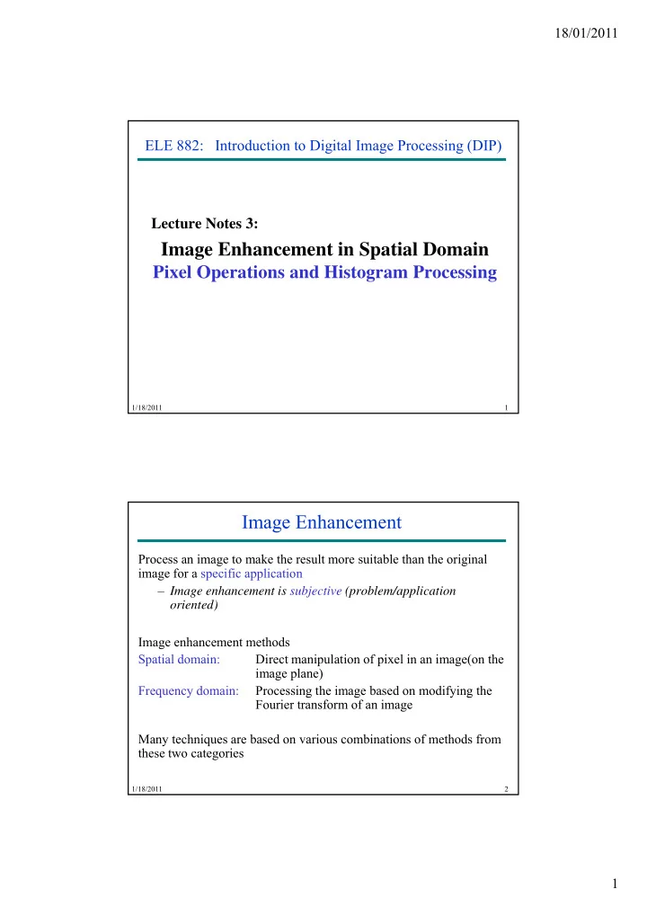
18/01/2011 ELE 882: Introduction to Digital Image Processing (DIP) Lecture Notes 3: 3 Image Enhancement in Spatial Domain Pixel Operations and Histogram Processing 1/18/2011 1 Image Enhancement Process an image to make the result more suitable than the original image for a specific application – Image enhancement is subjective (problem/application oriented) Image enhancement methods Spatial domain: Direct manipulation of pixel in an image(on the image plane) Frequency domain: q y Processing the image based on modifying the g g y g Fourier transform of an image Many techniques are based on various combinations of methods from these two categories 1/18/2011 2 1

18/01/2011 Image Enhancement Types of image enhancement operations Point/pixel operations O utput value at specific coordinates (x,y) is dependent only on the input value at (x y) (x,y). Local operations The output value at (x,y) is dependent on the input values in the neighborhood of (x,y). Global operations The output value at (x,y) is dependent on all the values in the input image. 1/18/2011 3 Basic concepts Spatial domain enhancement methods can be generalized as g ( x , y ) = T [ f ( x , y )] f ( x , y ) : input image g ( x , y ): processed (output) image T [*] : an operator on f (or a set of input images), defined over neighborhood of ( x , y ) Neighborhood about ( x , y ): a square or rectangular sub- image area centered at ( x , y ) 1/18/2011 4 2

18/01/2011 Basic Concepts 3x3 neighborhood about (x,y) 1/18/2011 5 Basic concepts g ( x , y ) = T [ f ( x , y )] Pixel/point operation: Neighborhood of size 1x1 : g depends only on f at ( x , y ) g p y ( , y ) g f T : a gray-level/intensity transformation/mapping function Let r = f ( x , y ) and s = g ( x , y ) r and s represent gray levels of f and g at ( x , y ) s = T ( r ) Then Local operations: g depends on the predefined number of neighbors of f at ( x , y ) Implemented by using mask processing or filtering Masks (filters, windows, kernels, templates) : a small (e.g. 3×3) 2-D array, in which the values of the coefficients determine the nature of the process 1/18/2011 6 3

18/01/2011 Common pixel operations  Image negatives  Log transformations  Power-law transformations 1/18/2011 7 Image negatives  Reverses the gray level order  For L gray levels the transformation function is s = T ( r ) = ( L - 1) - r s = T ( r ) = ( L 1) r Input image (X-ray image) Output image (negative) 1/18/2011 8 4

18/01/2011 Image negatives Application: To enhance the visibility for images with more dark portion Original digital mammogram Output image 1/18/2011 9 Image scaling s = T ( r ) = a. r (a is a constant) 1/18/2011 10 5

18/01/2011 Log transformations Function of s = c Log(1+ r ) 1/18/2011 11 Log transformations Properties of log transformations – For lower amplitudes of input image the range of gray levels is expanded expanded – For higher amplitudes of input image the range of gray levels is compressed Application: – This transformation is suitable for the case when the dynamic This transformation is suitable for the case when the dynamic range of a processed image far exceeds the capability of the display device (e.g. display of the Fourier spectrum of an image) – Also called “dynamic-range compression / expansion” 1/18/2011 12 6

18/01/2011 Log transformations Fourier spectrum with values of The result applying log transformation, range 0 to 1.5 x 10 6 scaled linearly c = 1 1/18/2011 13 Power-law Transformation Basic form: s = cr  , where c &  where c &  are positive Plots of equation Plots of equation s = cr   For various values of   c  1/18/2011 14 7

18/01/2011 Power-law Transformation For γ < 1: Expands values of dark pixels, compress values of brighter pixels For γ > 1: Compresses values of dark pixels, expand values of brighter pixels If γ =1 & c=1: Identity transformation (s = r) A variety of devices (image capture, printing, display) respond according to a power law and need to be corrected; Gamma ( γ ) correction The process used to correct the power-law response phenomena 1/18/2011 15 Power-law Transformation  Example of gamma correction  To linearize the CRT response a pre-distortion circuit is needed s = cr 1/  1/18/2011 16 8

18/01/2011 Gamma correction Linear Response of wedge gray CRT to Linear scale image wedge Gamma Output of corrected monitor wedge 1/18/2011 17 Power-law Transformation: Example MRI image of g Result of applying Result of applying Result of applying pp y g pp y g pp y g fractured human power-law power-law power-law spine transformation transformation transformation c = 1,  c = 1,  c = 1,  1/18/2011 18 9

18/01/2011 Power-law Transformation: Example Original Result of applying satellite power-law image image transformation transformation c = 1,  Result of Result of applying Result of applying applying power-law power-law transformation transformation c = 1,  c = 1,  1/18/2011 19 Piecewise-linear transformation Contrast stretching Goal: Increase the dynamic range of the gray levels for low contrast images Low-contrast images can result from – poor illumination poor illumination – lack of dynamic range in the imaging sensor – wrong setting of a lens aperture during image acquisition 1/18/2011 20 10

18/01/2011 Piecewise-linear transformation: contrast stretching Method where a 1 , a 2 , and a 3 control the result of contrast stretching if a 1 = a 2 = a 3 = 1 no change in gray levels if 1 h i l l if a 1 = a 3 = 0 and r 1 = r 2 , T (*) is a thresholding function, the result is a binary image 1/18/2011 21 Contrast Stretching Example Form of Original low- Transformation contrast image function Result of Result of contrast thresholding stretching 1/18/2011 22 11

18/01/2011 Bit Plane representation of 8-bit Image Bit Plane Example 12

18/01/2011 Bit Plane Example Histograms Histogram of an image with gray level (0 to L-1): A discrete function h ( r k ) = n k , where r k is the k th gray level and n k is the number of pixels in the image having gray level r k . How a histogram is obtained? H hi t i bt i d? – For B-bit image, initialize 2 B counters with 0 – Loop over all pixels x,y – When encountering gray level f ( x,y )= i, increment counter # i Normalized histogram: A discrete function p( r k ) = n k / n , where n is the total number of pixels in the image. p ( r k ) estimates probability of occurrence of gray-level r k  Distribution of gray-levels can be judged by measuring a histogram  Histogram provides global descriptions of the image (no local details)  Fewer, larger bins can be used to trade off amplitude resolution against sample size. 1/18/2011 26 13

18/01/2011 Example Histogram 1/18/2011 27 Example Histogram 1/18/2011 28 14

18/01/2011 Histogram Examples 1/18/2011 29 Contrast stretching through histogram If r max and r min are the maximum and minimum gray level of the input image and L is the total gray levels of output image The transformation function for contrast stretching will be     L      ( ) s T r r r   min   r r  max min r i r min r r max 0 L- 1 1/18/2011 30 15

18/01/2011 Histogram equalization  Idea: To find a non-linear transformation s = T ( r ) to be applied to each pixel of the input image f ( x y ) such that a to be applied to each pixel of the input image f ( x,y ) , such that a uniform distribution of gray levels in the entire range results for the output image g ( x,y ) .  Assuming ideal, continuous case, with normalized histograms     – that 0 1 0 1 r and s – T(r) is single valued i.e., there exists r= T -1 ( r ) – T(r) is monotonically increasing 1/18/2011 Center for Advance Studies in Engineering Digital Image Processing ECE6258 31 Histogram equalization A function T ( r ) is monotonically increasing if T ( r 1 ) < T ( r 2 ) for r 1 < r 2 , and monotonically decreasing if T ( r 1 ) > T ( r 2 ) for r 1 < r 2 . Example of a transformation function which is both single valued and monotonically increasing 1/18/2011 Center for Advance Studies in Engineering Digital Image Processing ECE6258 32 16

18/01/2011 Histogram equalization 1/18/2011 33 Histogram equalization 1/18/2011 34 17

18/01/2011 Histogram equalization examples Input image Output image Input histogram and cdf Output histogram and cdf 1/18/2011 Center for Advance Studies in Engineering Digital Image Processing ECE6258 35 Histogram equalization examples Low contrast image Output image Equalized histogram Equalized histogram high contrast image Output image 1/18/2011 Center for Advance Studies in Engineering Digital Image Processing ECE6258 36 18

18/01/2011 Histogram equalization examples Dark input image Output image Equalized histogram Equalized histogram Bright input image Output image 1/18/2011 Center for Advance Studies in Engineering Digital Image Processing ECE6258 37 Histogram equalization examples Transformation functions for histogram equalization 1/18/2011 Center for Advance Studies in Engineering Digital Image Processing ECE6258 38 19