Image Coding & Restoration . Dagstuhl 11/17/2016 1 - PowerPoint PPT Presentation
Gene Cheung National Institute of Informatics 17 th November, 2016 Graph Signal Processing for Image Coding & Restoration . Dagstuhl 11/17/2016 1 Acknowledgement Collaborators: Y. Mao, Y. Ji (NII, Japan) W. Hu, P. Wan, W. Dai, J.
Gene Cheung National Institute of Informatics 17 th November, 2016 Graph Signal Processing for Image Coding & Restoration . Dagstuhl 11/17/2016 1
Acknowledgement Collaborators: • Y. Mao, Y. Ji (NII, Japan) • W. Hu, P. Wan, W. Dai, J. Pang, J. Zeng, A. Zheng, O. Au (HKUST, HK) • Y.-H. Chao, A. Ortega (USC, USA) • D. Florencio, C. Zhang, P. Chou (MSR, USA) • Y. Gao, J. Liang (SFU, Canada) • L. Toni, A. De Abreu, P. Frossard (EPFL, Switzerland) • C. Yang, V. Stankovic (U of Strathclyde, UK) • X. Wu (McMaster U, Canada) • P. Le Callet (U of Nantes, France) • H. Zheng, L. Fang (USTC, China) • C.-W. Lin (National Tsing Hua University, Taiwan) • S. Yang, J. Liu, Z. Guo (Peking U. China) Dagstuhl 11/17/2016 2
Outline • Graph Signal Processing • Graph spectrum, GFT • PWS Image Coding using GFT • Prediction Residual Coding using GGFT • Image Denoising using Graph Laplacian Regularizer • Soft Decoding of JPEG Images w/ LERaG • Summary Dagstuhl 11/17/2016 3
Outline • Graph Signal Processing • Graph spectrum, GFT • PWS Image Coding using GFT • Prediction Residual Coding using GGFT • Image Denoising using Graph Laplacian Regularizer • Soft Decoding of JPEG Images w/ LERaG • Summary Dagstuhl 11/17/2016 4
Digital Signal Processing • Discrete signals on regular data kernels. • Ex.1: audio on regularly sampled timeline. • Ex.2: image on 2D grid. • Harmonic analysis tools (transforms, wavelets) for diff. tasks: • Compression. • Restoration. • Segmentation, classification. Dagstuhl 11/17/2016 5
Smoothness of Signals • Signals are often smooth . • Notion of frequency , band-limited . • Ex.: DCT : 1 N 1 cos X x n k k n 2 N n 0 2D DCT basis is set of outer-product of desired signal a x 1D DCT basis in x- and y-dimension. transform a transform coeff. 0 a 1 Typical pixel blocks have a 0 almost no high frequency components. Compact signal 0 representation Dagstuhl 11/17/2016 6
Graph Signal Processing • Signals on irregular data kernels described by graphs. • Graph: nodes and edges. • Edges reveals node-to-node relationships . example graph-signal 1. Data domain is naturally a graph. • Ex: ages of users on social networks. 2. Underlying data structure unknown. • Ex: images: 2D grid → structured graph. Graph Signal Processing (GSP) addresses the problem of processing signals that live on graphs. [1] D. I. Shuman et al.,” The Emerging Field of Signal Processing on Graphs: Extending High-dimensional Data Analysis to Networks 7 and other Irregular Domains ,” IEEE Signal Processing Magazine , vol.30, no.3, pp.83-98, 2013.
Graph Signal Processing Research questions* : • Sampling : how to efficiently acquire / node sense a graph-signal? edge • Graph sampling theorems. • Representation : Given graph-signal, how to compactly represent it? • Transforms, wavelets, dictionaries. • Signal restoration : Given noisy and/or partial graph-signal, how to recover it? • Graph-signal priors. 8 * Graph Signal Processing Workshop , Philadelphia, US, May 25-27, 2016. https://alliance.seas.upenn.edu/~gsp16/wiki/index.php?n=Main.Program
undirected graph w 1 1 Graph Fourier Transform (GFT) 1 , 2 1 2 3 4 0 0 0 w Graph Laplacian : 1 , 2 0 1 0 w 1 , 2 A • Adjacency Matrix A : entry A i,j has non-negative 0 1 0 1 0 0 1 0 edge weight w i,j connecting nodes i and j . 0 0 0 w 1 , 2 • Degree Matrix D : diagonal matrix w/ entry D i,i being 0 1 0 0 w 1 , 2 D 0 0 2 0 sum of column entries in row i of A . 0 0 0 1 D A 0 0 w w , , 1 , 2 1 , 2 i i i j 1 1 0 j w w 1 , 2 1 , 2 L • Combinatorial Graph Laplacian L : L = D-A 0 1 2 1 0 0 1 1 • L is symmetric (graph undirected). 2 L x x x x • L is a high-pass filter. 3 , : 2 3 4 • L is related to 2 nd derivative . 2 f x h f x f x h lim f x 2 h 0 h *https://en.wikipedia.org/wiki/Second_derivative 9
Graph Spectrum from GFT • Graph Fourier Transform (GFT) is eigen-matrix of graph Laplacian L . w eigenvalue 1 1 … 1 , 2 1 2 3 4 8 L u u eigenvector i i i 1st AC eigenvector 1. Edge weights affect shapes of eigenvectors. 2. Eigenvalues (≥ 0) as graph frequencies . • Constant eigenvector is DC. • # zero-crossings increases as λ increases. • GFT defaults to DCT for un-weighted connected line. • GFT defaults to DFT for un-weighted connected circle. Dagstuhl 11/17/2016 10
Variants of Graph Laplacians • Graph Fourier Transform (GFT) is eigen-matrix of graph Laplacian L . eigenvalue L u u eigenvector i i i • Other definitions of graph Laplacians: Characteristics: • Normalized graph Laplacian: • Normalized. • Symmetric. 1 / 2 1 / 2 1 / 2 1 / 2 L n D LD I D AD • No DC component. • Random walk graph Laplacian: • Normalized. • 1 1 Asymmetric. L rw D L I D A • Eigenvectors not orthog. • Generalized graph Laplacian [1]: • Symmetric. • L plus self loops. * L g L D • Defaults to DST, ADST. [1] Wei Hu, Gene Cheung, Antonio Ortega, " Intra-Prediction and Generalized Graph Fourier Transform for Image Coding ," IEEE Signal Processing Letters , vol.22, no.11, pp. 1913-1917, November 2015. 11
GSP and Graph-related Research GSP: SP framework that unifies concepts from multiple fields. Laplace- Laplace Partial Differential Beltrami Computer Graphics equation Eq’ns operator Computer graphical model, spectral Graph Signal manifold learning, clustering Vision Machine classifier learning Processing* (GSP) Learning DSP eigen-analysis of Max cut, graph graph Laplacian, transformation adjacency matrices Combinatorial Spectral Graph Theory Graph Theory Dagstuhl 11/17/2016 12
Outline • Graph Signal Processing • Graph spectrum, GFT • PWS Image Coding using GFT • Prediction Residual Coding using GGFT • Image Denoising using Graph Laplacian Regularizer • Soft Decoding of JPEG Images w/ LERaG • Summary Dagstuhl 11/17/2016 13
PWS Image Compression using GFT • DCT are fixed basis. Can we do better? • Idea : use adaptive GFT to improve sparsity [3]. 1. Assign edge weight 1 to adjacent pixel pairs. 2. Assign edge weight 0 to sharp signal discontinuity. 3. Compute GFT for transform coding, transmit coeff. GFT α x 4. Transmit bits ( contour ) to identify chosen GFT to decoder (overhead of GFT). Shape-adaptive wavelets [1] G. Shen et al., “ Edge-adaptive Transforms for Efficient Depth Map Coding ,” can also be done. IEEE Picture Coding Symposium , Nagoya, Japan, December 2010. [2] M. Maitre et al., “ Depth and depth-color Coding using Shape-adaptive Wavelets ,” 14 Journal of Visual Communication and Image Representation , vol.21, July 2010, pp.513-522.
Transform Comparison Transform Representation Transform Description “Sparsest” signal representation given Karhunen-Loeve Can be expensive (if poorly available data / statistical model Transform (KLT) structured) non-sparse signal representation Discrete Cosine little (fixed transform) across sharp boundaries Transform (DCT) minimizes the total rate of signal’s transform representation & Graph Fourier Transform (GFT) transform description [1] Wei Hu, Gene Cheung, Antonio Ortega, Oscar Au, " Multiresolution Graph Fourier Transform for Compression of 15 Piecewise Smooth Images ," IEEE Transactions on Image Processing , vol.24, no.1, pp.419-433, January 2015.
MR-GFT: Definition of the Search Space for Graph Fourier Transforms Rate of transform coefficient vector Rate of transform description T • In general, weights could be any number in [0,1] • To limit the description cost • Restrict weights to a small discrete set strong Histogram of inter-pixel difference 3500 - "1": s trong correlation in smooth regions 3000 - "0": zero correlation in sharp boundaries 2500 zero - "c": weak correlation in slowly-varying parts 2000 1500 1000 weak 500 16 16 0 0 5 10 15 20 25 30 35 40 45 50
MR-GFT: Derivation of Optimal Edge Weights for Weak Correlation • Assume a 1D 1st-order autoregressive (AR) process where, non-zero mean RV smooth jump w 1 1 , k k … … non-zero mean random var. 1 2 k N k-1 • Assuming the only weak correlation exists between and k th row mean vector Dagstuhl 11/17/2016 17 k-th
Recommend
More recommend
Explore More Topics
Stay informed with curated content and fresh updates.

![Image and Video Coding: Hybrid Video Coding s n 1 [ x , y ] s n [ x , y ] m k = ( m x , m](https://c.sambuz.com/761427/image-and-video-coding-hybrid-video-coding-s.webp)
